Farewell to the Rotating-Wave Approximation: An Exact Solution of the Quantum Rabi Model

1. Introduction

In the early days of quantum mechanics, Rabi proposed the Rabi model to treat the interaction between an electromagnetic field and an atom. Since this model quantized only the atom, rather than the electromagnetic wave, it could explain many phenomena (such as Rabi oscillations), but could not explain phenomena involving quantization of the electromagnetic field, such as spontaneous emission.

To explain spontaneous emission and other phenomena involving quantization of the electromagnetic field, Jaynes and Cummings proposed the Quantum Rabi Model (QRM) in 1962. This model also quantizes the electromagnetic field, meaning that vacuum fluctuations of the electromagnetic field cannot be neglected. Thus, spontaneous emission is simply “stimulated emission” “excited” by vacuum fluctuations of the electromagnetic field.

However, for quite a long time after the QRM was proposed, people believed that it had no exact solution, and that an exact solution existed only after applying the rotating-wave approximation (RWA). The model after applying the rotating-wave approximation is called the Jaynes-Cummings model (JCM).

The JCM successfully explains phenomena such as spontaneous emission and vacuum Rabi oscillations, but because it uses the rotating-wave approximation, it still cannot explain phenomena such as the Lamb shift. Moreover, strong coupling can now be realized in Circuit QED systems. When the coupling becomes very strong, the rotating-wave approximation fails, and the JCM deviates substantially from experimental results. Clearly, the QRM is still needed in some cases.

Surprisingly, an exact solution of the QRM was not found until 2011 [1]. Since then, people have also become interested in exact solutions of various generalized quantum Rabi models, such as extensions to multiple atoms (the Dicke model) and multiple field modes.

This article derives the exact solution of the QRM, with the following structure:

Section 2: Introduce the Hamiltonians of the QRM and JCM

Section 3: Briefly derive the exact solution of the JCM

Section 4: Derive the exact solution of the QRM

Section 5: Introduce the conserved quantities and symmetries of the JCM and QRM

2. Hamiltonians of the QRM and JCM

The quantum Rabi model (QRM) describes the interaction between a single-mode optical field and a two-level system.

Let the Hilbert space of the single-mode optical field be \(\mathcal{H} \cong L^{2}(\mathbb{R})\), and the Hilbert space of the two-level system be \(\mathcal{K} \cong \mathbb{C}^2\). Then the QRM Hamiltonian \(H\in \mathcal{L}(\mathcal{H}\otimes \mathcal{K})\) is given by:

\[\begin{aligned} H&= \underbrace{\omega \left(a^\dag a+\frac{1}{2}\right)}_{\text{field}}+ \underbrace{ \frac{\Delta}{2} \sigma_z}_{\text{atom}} + \underbrace{g\sigma_x(a+a^\dag)}_{\text{atom-field coupling}} \\&= \underbrace{\omega \left(a^\dag a+\frac{1}{2}\right)}_{\text{field}}+ \underbrace{ \frac{\Delta}{2} \sigma_z}_{\text{atom}} + \underbrace{g(\sigma_++\sigma_-)(a+a^\dag)}_{\text{atom-field coupling}} \end{aligned}\]

Here, \(a^\dag , a\) are the creation and annihilation operators on \(\mathcal{H} \), and \(\sigma_z, \sigma_{\pm}\) are the Pauli Z operator and raising and lowering operators on \(\mathcal{K}\). \(g\) is called the Rabi frequency, and it measures the coupling strength between the optical field and the two-level system.

If we discard the terms with large energy differences, \(\sigma_- a\) and \(\sigma_+ a^\dag\), we obtain the Hamiltonian of the Jaynes-Cummings model (JCM):

\[\begin{aligned} H&= \underbrace{\omega \left(a^\dag a+\frac{1}{2}\right)}_{\text{field}}+ \underbrace{ \frac{\Delta}{2} \sigma_z}_{\text{atom}} + \underbrace{g(\sigma_+ a + \sigma_- a^{\dag})}_{\text{atom-field coupling}}\end{aligned}\]

This is the rotating-wave approximation. The discarded terms are called counter-rotating terms, while the retained terms are called co-rotating terms.

The rotating-wave approximation is justified because the energy difference between the two levels involved in the counter-rotating terms is \(\omega + \Delta\), which is much greater than the energy difference \(|\omega - \Delta|\) of the co-rotating terms. The exponential factor involved in the former is \(e^{\pm\mathrm{i} (\omega + \Delta) t}\), while that in the latter is \(e^{\pm\mathrm{i}(\omega-\Delta)}t\). Since \(e^{\pm\mathrm{i} (\omega + \Delta) t}\) varies too rapidly, it can be regarded as averaging to zero and eliminated.

In addition, this can also be seen from perturbative calculations: the terms obtained after perturbative calculations are proportional to the inverse of the energy difference, namely \(\frac{1}{\omega +\Delta}\) for the former and \(\frac{1}{|\omega - \Delta|}\) for the latter. Since \(\frac{1}{\omega + \Delta}\) is much smaller than \(\frac{1}{|\omega - \Delta|}\), the former can be neglected.

2. Exact Solution of the JCM

We can expand \(H\) in the photon-number representation:

\[\begin{aligned} H &= \color{gray}{ \begin{matrix} |g,0\rangle \\ |e,0\rangle \\ |g,1\rangle \\ |e,1\rangle \\ |g,2\rangle \\ \vdots \end{matrix} } \begin{bmatrix} 1 & 0 & 0 & 0 & 0 & \cdots \\ 0 & 1 & 0 & 0 & 0 & \cdots \\ 0 & 0 & 3 & 0 & 0 & \cdots \\ 0 & 0 & 0 & 3& 0 & \cdots \\ 0 & 0 & 0 & 0 & 5& \cdots \\ \vdots & \vdots & \vdots & \vdots & \vdots & \ddots \end{bmatrix} \frac{\omega}{2}+\begin{bmatrix} -1 & 0 & 0 & 0 & 0 & \cdots \\ 0 & 1 & 0 & 0 & 0 & \cdots \\ 0 & 0 & -1 & 0 & 0 & \cdots \\ 0 & 0 & 0 & 1 & 0 & \cdots \\ 0 & 0 & 0 & 0 & -1 & \cdots \\ \vdots & \vdots & \vdots & \vdots & \vdots & \ddots \end{bmatrix} \frac{\Delta}{2} +\begin{bmatrix} 0 & 0 & 0 & 0 & 0 & \cdots \\ 0 & 0 & 1 & 0 & 0 & \cdots \\ 0 & 1 & 0 & 0 & 0 & \cdots \\ 0 & 0 & 0 & 0 & \sqrt{2} & \cdots \\ 0 & 0 & 0 & \sqrt{2} & 0 & \cdots \\ \vdots & \vdots & \vdots & \vdots & \vdots & \ddots \end{bmatrix} g \end{aligned} \]

Here, \(g,e\) represent the ground state and excited state of the two-level system, respectively, and \(0,1,2,\cdots\) represents the number of excitations in the optical field (i.e., the photon number).

It can be further written as:

\[\begin{aligned} H = \bigoplus_{n=1}^\infty \begin{bmatrix} n\omega+\frac{\Delta}{2} & g\sqrt{n} \\ g\sqrt{n} & (n+1)\omega -\frac{\Delta}{2} \end{bmatrix} \end{aligned}\]

Here, \(n\) represents the total excitation number, namely the sum of the excitation number of the two-level system and that of the optical field (i.e., the photon number).

This matrix can clearly be diagonalized exactly, with eigenvalues \(\left(n+ \frac{1}{2}\right)\omega \pm \sqrt{\left(\frac{\omega - \Delta}{2}\right)^2 + ng^2}\). Let \(\Delta_n = \sqrt{\left(\frac{\omega - \Delta}{2}\right)^2 + ng^2}\); then the energy levels are \(E_{\pm,n} = \left(n + \frac{1}{2}\right)\omega \pm \frac{\Delta_n}{2}\).

The eigenstates at these energy levels are called dressed states:

\[\begin{aligned} |-,n\rangle &= \cos \theta_n |e,n-1\rangle - \sin \theta_n |g,n\rangle \\ |+,n\rangle &= \sin \theta_n |e,n-1\rangle + \cos \theta_n |g,n\rangle \end{aligned}\]

where

\[\begin{aligned} \cos \theta_n &= \frac{2\sqrt{n}g}{\sqrt{(\Delta_n-\Delta_0)^2 + 4ng^2}} \\ \sin \theta_n &= \frac{\Delta_n-\Delta_0}{\sqrt{(\Delta_n-\Delta_0)^2 + 4ng^2}} \end{aligned}\]

and \(\Delta _0 := \Delta - \omega\).

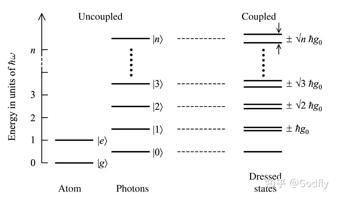
Schematic energy-level diagram of dressed states. This figure corresponds to the zero-detuning case (\(\omega = \Delta\)), where \(g\_0:=g\) is the Rabi frequency. Image source: Internet

4. Exact Solution of the QRM

Next, we derive the exact solution of the QRM following the method of a 2012 paper [2]. Compared with the earliest method in the 2011 paper [1], it is more suitable for physicists rather than mathematicians.

Expanding the QRM Hamiltonian in the basis \(\{|+\rangle, |-\rangle\} =\left\{\frac{|e\rangle + |g\rangle}{\sqrt{2}} ,\frac{|e\rangle - |g\rangle}{\sqrt{2}}\right\}\) gives:

\[H = \begin{bmatrix} \omega a^\dag a + g(a+a^\dag) & \Delta/2 \\ \Delta/2 & \omega a^\dag a + g(a-a^\dag) \end{bmatrix}\]

It can be verified that \(H = [\omega a^\dag a + g(a+a^\dag)] |+\rangle\langle+| + [\omega a^\dag a - g(a+a^\dag)] |-\rangle\langle-| + \frac{\Delta}{2}(|+\rangle\langle-| + |-\rangle\langle+|)\)

Perform the Bogoliubov transformation \(A = a +g/\omega,\,B=a-g/\omega\), and define Extended Fock states:

\[|0\rangle_A=e^{-\frac{g}{\omega}(a^\dag - a)} |0\rangle = |\frac{-\omega}{g}\rangle\]\[|n\rangle_A = \frac{A^{\dag n}}{\sqrt{n!}} |0\rangle_A\]

Note that \(|0\rangle_A\) is a coherent state with parameter \(-\frac{\omega}{g}\).

It can be verified that \([A,A^\dag]=1\). Therefore, relations that hold for ordinary Fock states also hold for Extended Fock states:

\[A|n\rangle_A = \sqrt{n} |n-1\rangle_A\]\[A^\dag |n\rangle_A = \sqrt{n+1} |n + 1\rangle_A\]

We then have

\[H = \begin{bmatrix} \omega A^\dag A - g^2 /\omega& \Delta/2 \\ \Delta/2 & \omega A^\dag A - 2g(A+A^\dag) + 3g^2/\omega \end{bmatrix}\]

Suppose the eigenstate is:

\[|\psi\rangle=\begin{bmatrix} \sum \sqrt{n!} e_n |n\rangle_A \\ \sum \sqrt{n!} f_n |n\rangle_A \end{bmatrix}\]

Substituting into \(H|\psi\rangle = E|\psi\rangle\) gives:

\[\begin{cases} e_n = -\frac{\Delta/2}{ n\omega -g^2/\omega - E} f_n \\ nf_n = \Omega(n-1) f_{n-1} - f_{n-2} \end{cases}\]

where \(\Omega(n) = \frac{2g}{\omega}+\frac{1}{2g}\left[ n\omega - g^2/\omega -E - \frac{(\Delta/2)^2}{n\omega - g^2/\omega - E}\right]\)

Similarly, the Hamiltonian can also be written as:

\[H = \begin{bmatrix} \omega B^\dag B -2g(B + B^\dag) + 3g^2 & \Delta/2 \\ \Delta/2 & \omega B^\dag B - g^2/\omega \end{bmatrix}\]

Suppose the eigenstate is

\[|\psi^\prime\rangle=\begin{bmatrix} \sum \sqrt{n!} (-1)^nf_n^\prime |n\rangle_B \\ \sum \sqrt{n!} (-1)^ne_n^\prime |n\rangle_B \end{bmatrix}\]

Substituting into \(H|\psi\rangle = E|\psi\rangle\) gives:

\[\begin{cases} e_n^\prime = -\frac{\Delta/2}{n\omega - g^2/\omega -E} f^\prime_n \\ nf^\prime_n = \Omega(n-1)f^\prime_{n-1} - f_{n-2} \end{cases}\]

It can be seen that \(f_n\) and \(f_n^\prime\), as well as \(e_n\) and \(e_n^\prime\), satisfy the same recurrence relation. Let \(f_0 = f_0^\prime = 1\), then \(f_n = f_n^\prime\), \(e_n = e_n^\prime\).

Since the two eigenstates \(|\psi \rangle, |\psi^\prime\rangle\) must be proportional, \(|\psi^\prime\rangle = \kappa |\psi\rangle\), where \(\kappa \in \mathbb{C}\), we have:

\[\begin{cases} \sum \sqrt{n!} (-1)^nf_n |n\rangle_B = \kappa \sum \sqrt{n!} e_n |n\rangle_A \\ \sum \sqrt{n!} (-1)^ne_n |n\rangle_B = \kappa\sum \sqrt{n!} f_n |n\rangle_A \end{cases}\]

Left-multiplying both sides by the vacuum state \(\langle0|\), and using

\[\begin{aligned} \sqrt{n!}\langle 0 | n\rangle_A &= \langle 0 |A^{\dag n}|0\rangle_A \\&= \langle 0|(a+\lambda)^\dag | 0 \rangle_A \\&= \lambda^n\langle 0|0\rangle_A \\&= \lambda^n e^{-\lambda^2/2} \end{aligned}\]\[\sqrt{n!} \langle 0|n\rangle_B = (-\lambda)^n e^{-\lambda^2/2}\]

where \(\lambda = g/\omega\).

Thus:

\[\begin{cases} \sum \lambda^n e^{-\lambda^2/2} f_n = \kappa \sum \lambda^n e^{-\lambda^2/2} e_n \\ \sum\lambda^n e^{-\lambda^2/2}e_n = \kappa\sum \lambda^n e^{-\lambda^2/2} f_n \end{cases}\]\[\Rightarrow \left(\sum \lambda^n e^{-\lambda^2/2} f_n\right)^2 = \left(\sum\lambda^n e^{-\lambda^2/2} e_n \right)^2 \]\[\Rightarrow \sum \lambda^n e^{-\lambda^2/2} (f_n \pm e_n )= 0\]\[\begin{aligned} \Rightarrow \sum \lambda^n e^{-\lambda^2/2} f_n \left(1\pm \frac{\Delta/2}{n\omega - g\lambda -E}\right) = 0 \end{aligned}\]

Let \(G_{\pm}(x) = \sum f_n \lambda^n \left(1\mp \frac{\Delta}{2\omega(x+\lambda^2-n)}\right)\); it is a transcendental function.

Clearly, the zeros of \(G_{\pm}(x) \) are the eigenenergy levels (in units of \( \omega\)).

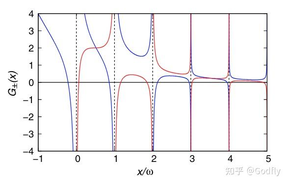
Zeros of \(G\_{\pm}(x)\). Image source: [1]

The eigenstates are:

\[\begin{aligned} &\phantom{=}\sum_n\left[ \sqrt{n!} f_n |n\rangle_B \otimes \frac{|e\rangle + |g\rangle}{\sqrt{2}} + \sqrt{n!} e_n |n\rangle_B \otimes \frac{|e\rangle - |g\rangle}{\sqrt{2}}\right] \\&=\sum_n \left[ \sqrt{n!/2} (f_n - e_n)\right] |n\rangle_B \otimes |g\rangle + \sum_n \left[ \sqrt{n!/2} (f_n + e_n)\right] |n\rangle_B \otimes |e\rangle \\&=\sum_n \left[ \sqrt{\frac{n!}{2}} f_n \left(1 - \frac{\Delta/2}{n\omega - g\lambda -E}\right)\right] |n\rangle_B \otimes |g\rangle + \sum_n \left[ \sqrt{\frac{n!}{2}} f_n \left(1 + \frac{\Delta/2}{n\omega - g\lambda - E}\right) \right] |n\rangle_B \otimes |e\rangle \end{aligned}\]

At this point, we have obtained the exact solution for the energy levels and eigenstates of the QRM Hamiltonian. A schematic diagram of the energy levels as a function of coupling strength is shown below:

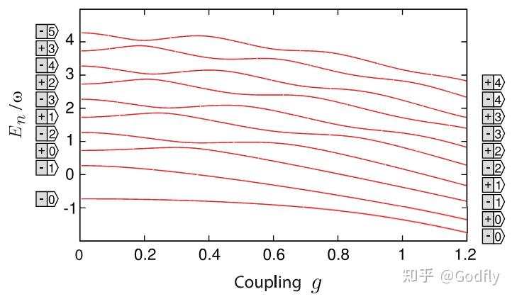
Transition from the JCM to the QRM. The labels on the left are JCM eigenstates, while those on the right are QRM eigenstates. Image source: [1]

As can be seen from the figure, as the coupling coefficient increases, the energy gap between the ground state and the first excited state decreases. This is the Lamb shift. However, the Lamb shift usually refers to the interaction between an atom and a vacuum optical field with multiple modes, rather than the single-mode optical field discussed here.

In addition, as the coupling coefficient increases, energy levels that would originally cross in the JCM do not cross in the QRM; instead, they first approach each other and then move apart. This is the so-called avoided crossing.

5. Conserved Quantities and Symmetries

The JCM has the conserved quantity \(N = a^\dag a+\sigma_+\sigma_- = a^\dag a + (\mathbb{I} + \sigma_z)/2\), whose eigenvalues are \(n=0,1,2,\cdots\), \(N|\pm,n\rangle = \left(n + \frac{1\pm 1}{2}\right)|\pm,n\rangle\). The physical meaning of this conserved quantity is the total number of excitations.

The conserved quantity \(N\) generates a continuous \(U(1)\) symmetry. This is because \([N,H] = 0 \Rightarrow [e^{-\mathrm{i\theta}N},H]=0\). In other words, the Hamiltonian remains unchanged after the following transformations:

\[a \rightarrow e^{-\mathrm{i}\theta N} a e^{\mathrm{i}\theta N} = a e^{-\mathrm{i}\theta}\]\[a^\dag \rightarrow e^{-\mathrm{i}\theta N} a^\dag e^{\mathrm{i}\theta N} = a^\dag e^{\mathrm{i}\theta}\]\[\sigma_{\pm} \rightarrow e^{-\mathrm{i}\theta N} \sigma_{\pm} e^{\mathrm{i}\theta N} = \sigma_\pm e^{\pm\mathrm{i}\theta}\]

The conserved quantity of the QRM is \(\Pi = e^{-\mathrm{i}\pi N} = -\sigma_+\sigma_- \otimes e^{\mathrm{i}\pi a^\dag a}\), whose eigenvalues are \(\pm 1\), \(\Pi |\pm,n\rangle = \mp (-1)^n |\pm,n\rangle\).

Although the QRM loses \(U(1)\) symmetry, it still has a discrete \(Z_2\) symmetry. This is because \([\Pi,H]=0\), so that the Hamiltonian remains unchanged after the following transformations:

\[a \rightarrow \Pi a \Pi^\dag = -a\]\[a^\dag \rightarrow \Pi a^\dag \Pi^\dag = -a^\dag\]\[\sigma_\pm \rightarrow \Pi \sigma_\pm \Pi^\dag = -\sigma_\pm\]

The \(Z_2\) symmetry can be regarded as the \(U(1)\) symmetry being broken from \(\theta \in [0,2\pi)\) to \(\theta \in \{0,\pi\}\). This can also be seen intuitively from the Hamiltonian: the JCM contains only co-rotating terms and thus has continuous \(U(1)\) symmetry, whereas the QRM contains both co-rotating and counter-rotating terms. These two terms can meet only at \(\theta \in \{0,\pi\}\), so there is only discrete \(Z_2\) symmetry.

References

1. ^abBraak, D. Integrability of the Rabi Model. Phys. Rev. Lett. 2011, 107 (10), 100401. https://doi.org/10.1103/PhysRevLett.107.100401
2. ^Chen, Q.-H.; Wang, C.; He, S.; Liu, T.; Wang, K.-L. Exact Solvability of the Quantum Rabi Model Using Bogoliubov Operators. Phys. Rev. A 2012, 86 (2), 023822. https://doi.org/10.1103/PhysRevA.86.023822