A Fully Quantum Theory of Lasers
 Haifei
Most materials introducing lasers derive them in a classical or semiclassical form. So what does a fully quantum theory of lasers look like? And what is it useful for?
This article briefly introduces the Scully-Lamb theory of lasers. It is a fully quantum theory, and since it is generally introduced only in the final chapters of quantum optics textbooks, while (semi-)classical theories work well in most cases, not many people are familiar with the Scully-Lamb theory.
The Scully-Lamb theory makes more accurate predictions for the photon-number distribution when the pump strength is below or near threshold, which (semi-)classical theories cannot do.
This article is structured as follows:
Section 1 introduces the Jaynes-Cummings model, which handles the interaction between the optical field and a two-level system.
Section 2 introduces the Lindblad master equation, which handles the interaction between the optical field and a thermal reservoir.
Section 3 derives the Scully-Lamb theory. It is simply the result of the combined action of the Jaynes-Cummings model and the Lindblad master equation.
For simplicity, this article sets \(\hbar = 1\) 。
1. Jaynes-Cummings Model (JCM)
(Those familiar with the JCM may skip this section.)
The JCM describes the coupling between a single-mode optical field and a two-level system. Since it also quantizes the optical field, it is a fully quantum model.
In addition to quantizing the optical field, the JCM also makes the dipole approximation (Dipole Approximation) and the rotating-wave approximation (Rotating-Wave Approximation, RWA) in order to facilitate its solution. This process is beyond the scope of this article; interested readers may consult textbooks and online materials.
Let the Hilbert space of the single-mode optical field be \(\mathcal{H} \cong L^{2}(\mathbb{R})\) and that of the two-level system be \(\mathcal{K} \cong \mathbb{C}^2\). Then the Jaynes-Cumming Hamiltonian \(H \in \mathcal{L}(\mathcal{H}\otimes \mathcal{K})\) is given by:
\[\begin{aligned} H&= \underbrace{\omega \left(a^\dag a+\frac{1}{2}\right)}_{\text{field}}+ \underbrace{\omega_a \frac{\sigma_z}{2}}_{\text{atom}} + \underbrace{\Omega(\sigma_+ a + \sigma_- a^{\dag})}_{\text{atom-field coupling}} \\ &= \underbrace{\omega \left(a^\dag a+\frac{1}{2}+\frac{\sigma_z}{2}\right)}_{H_0} + \underbrace{\frac{\Delta}{2} \sigma_z + \Omega(\sigma_+ a + \sigma_- a^{\dag})}_{H_\text{I}} \end{aligned}\]Here, \(a^\dag , a\) are the creation and annihilation operators on \(\mathcal{H}\), while \(\sigma_z, \sigma_{\pm}\) are the Pauli Z operator and the raising and lowering operators on \(\mathcal{K}\). \(\Omega\) is called the Rabi frequency, and it measures the coupling strength between the optical field and the two-level system.
1.1 Diagonalization of the JCM
Since \(H_0\) contains only diagonal terms, we can separate it from the solution: let \(|\psi\rangle = e^{-\mathrm{i}H_0t} |\psi_\text{I}\rangle\), then \(\mathrm{i} \frac{\mathrm{d}}{\mathrm{d}t}|\psi_\text{I}\rangle = H_\text{I}|\psi_\text{I}\rangle\). Therefore, we need only study \(H_\text{I}\). This method is called the interaction picture.
We can expand \(H_\text{I}\) in the photon-number basis:
\[\begin{aligned} H_\text{I} &= \color{gray}{ \begin{matrix} |g,0\rangle \\ |e,0\rangle \\ |g,1\rangle \\ |e,1\rangle \\ |g,2\rangle \\ \vdots \end{matrix} } \begin{bmatrix} 0 & 0 & 0 & 0 & 0 & \cdots \\ 0 & 0 & 1 & 0 & 0 & \cdots \\ 0 & 1 & 0 & 0 & 0 & \cdots \\ 0 & 0 & 0 & 0 & \sqrt{2} & \cdots \\ 0 & 0 & 0 & \sqrt{2} & 0 & \cdots \\ \vdots & \vdots & \vdots & \vdots & \vdots & \ddots \end{bmatrix}\Omega+ \begin{bmatrix} -1 & 0 & 0 & 0 & 0 & \cdots \\ 0 & 1 & 0 & 0 & 0 & \cdots \\ 0 & 0 & -1 & 0 & 0 & \cdots \\ 0 & 0 & 0 & 1 & 0 & \cdots \\ 0 & 0 & 0 & 0 & -1 & \cdots \\ \vdots & \vdots & \vdots & \vdots & \vdots & \ddots \end{bmatrix} \frac{\Delta}{2} \end{aligned} \]where \(g,e\) respectively denote the ground state and excited state of the two-level system, and \(0,1,2,\cdots\) denotes the excitation number of the optical field (i.e., the photon number).
It can be further written as:
\[\begin{aligned} H_\text{I} = \bigoplus_{n=1}^\infty \begin{bmatrix} \frac{\Delta}{2} & \Omega\sqrt{n} \\ \Omega\sqrt{n} & -\frac{\Delta}{2} \end{bmatrix} \end{aligned}\]where \(n\) denotes the total excitation number, namely the sum of the excitation number of the two-level system and that of the optical field (i.e., the photon number).
This matrix can clearly be diagonalized exactly, with eigenvalues \(\pm \sqrt{\left(\frac{\Delta}{2}\right)^2 + n\Omega^2}\). Let \(\Delta_n = \sqrt{\Delta^2 + 4n\Omega^2}\); then the energy levels in the original picture (i.e., the non-interaction picture) are \(E_{\pm,n} = \omega \left(n + \frac{1}{2}\right) \pm \frac{\Delta_n}{2}\).
The eigenstates at these energy levels are called dressed states:
\[\begin{aligned} |-,n\rangle &= \cos \theta_n |e,n-1\rangle - \sin \theta_n |g,n\rangle \\ |+,n\rangle &= \sin \theta_n |e,n-1\rangle + \cos \theta_n |g,n\rangle \end{aligned}\]where
\[\begin{aligned} \cos \theta_n &= \frac{2\sqrt{n}\Omega}{\sqrt{(\Delta_n-\Delta)^2 + 4n\Omega^2}} \\ \sin \theta_n &= \frac{\Delta_n-\Delta}{\sqrt{(\Delta_n-\Delta)^2 + 4n\Omega^2} }\end{aligned}\]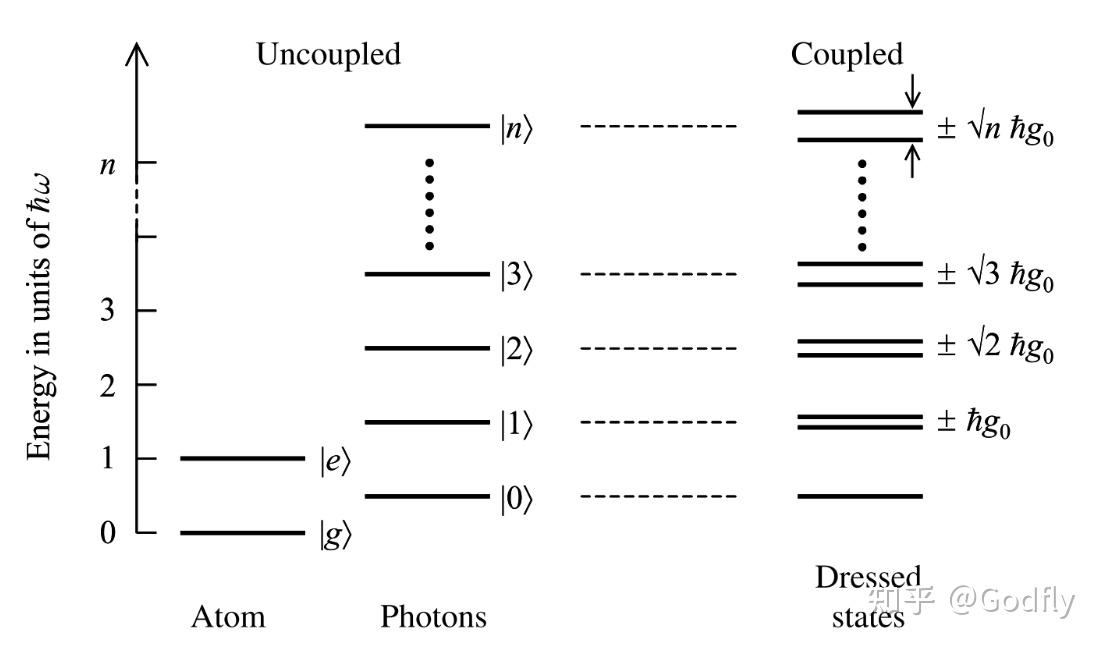
Schematic energy-level diagram of dressed states. This figure corresponds to the zero-detuning case (\(\Delta=0\)), where \(g\_0:=\Omega\) is the Rabi frequency.
1.2 Optical Field Evolution under the JCM
Since we are ultimately concerned only with the quantum state of the optical field, we take a partial trace over the atomic part. Suppose that the initial atomic state is \(|e\rangle\langle e|\). Then, after time \(\tau\), the optical field evolves into
\[\rho \rightarrow F(\tau) \rho := \text{tr}_\text{a}[e^{-\mathrm{i}H \tau} (|e\rangle\langle e|\otimes \rho) e^{\mathrm{i}H\tau}]\]where \(H\) is the JCM Hamiltonian, and \(\text{tr}_\text{a}\) denotes the partial trace over the atomic system.
Let us first examine how \(|n\rangle\) evolves under \(F(\tau)\), i.e., calculate \(F(\tau)(|n\rangle\langle n|)\):
\[\begin{aligned} |e,n\rangle &= \cos \theta_n | -,n+1\rangle + \sin \theta_n |+,n+1\rangle \\ e^{-\mathrm{i}H\tau} |e,n\rangle &= \cos \theta_n e^{-\mathrm{i} \frac{\Delta_{n+1}}{2}\tau} |-,n+1\rangle + \sin \theta_n e^{\mathrm{i} \frac{\Delta_{n+1}}{2}\tau}|+,n+1\rangle \\ &= \cos \theta_n e^{-\mathrm{i} \frac{\Delta_{n+1}}{2}\tau} (\cos \theta_n |e,n\rangle - \sin \theta_n |g,n + 1\rangle)\\&\phantom{=}+ \sin \theta_n e^{\mathrm{i} \frac{\Delta_{n+1}}{2}\tau}(\sin \theta_n |e,n\rangle + \cos \theta_n |g,n+1\rangle) \\ &= C_{e,n} |e,n\rangle + C_{g, n+1} | g, n+1\rangle \\ \text{tr}_\text{atom}[e^{-\mathrm{i}H\tau}|e,n\rangle\langle e,n|e^{\mathrm{i}H\tau}] &=|C_{e,n}|^2 |n\rangle\langle n| + |C_{g,n+1}|^2 |n+1\rangle\langle n+1| \end{aligned}\]where
\[\begin{aligned} C_{e,n} &= \cos(\Delta_{n+1} \tau /2) + \mathrm{i} \cos(2\theta_n)\sin(\Delta_{n+1} \tau/2)\\ C_{g,n+1} &= \mathrm{i} \sin (2\theta_n) \sin (\Delta_{n+1} \tau/2) \end{aligned}\]Suppose that the initial state of the optical field is a photon-number mixed state \(\rho = \sum_n p_n |n\rangle\langle n|\). Then
\[\begin{aligned} F(\tau) \rho &= \sum_n p_n F(\tau)(|n\rangle\langle n|)\\ &= \sum_n p_n [|C_{e,n}|^2 |n\rangle\langle n | + |C_{g,n+1}|^2 |n+1\rangle\langle n+1|] \\ &= \sum_n p_n |C_{e,n}|^2 |n\rangle\langle n | + \sum_{n=1} p_{n-1} |C_{g,n}|^2 |n\rangle\langle n| \end{aligned}\]Thus, the new \(p_n^\prime = \langle n|F(\tau) \rho |n\rangle\) is
\[\begin{aligned} \langle n|F(\tau) \rho |n\rangle &= |C_{e,n}|^2 p_n + |C_{g,n}|^2 p_{n-1} \\ &=: (1-C_n) p_n + C_{n-1} p_{n-1} \end{aligned}\]where \(C_n := |C_{g,n+1}|^2 \Rightarrow 1-C_n = |C_{e,n}|^2\).
We will use the expression for \(\langle n|F(\tau) \rho |n\rangle\) later.
There is also \(C_{n-1} = |C_{g,n}|^2=\sin^2 (2\theta_n) \sin^2 \left(\frac{\Delta_{n}}{2} \tau\right) = \frac{4n\Omega^2}{4n\Omega^2+\Delta_n^2} \sin^2 \left(\frac{\Delta_{n}}{2} \tau\right)\), which will also be useful later.
Summary: This section obtained the analytical solution of the Jaynes-Cummings model. Given a coupled system consisting of a two-level atom and an optical field, with initial state \(\rho\), we can find its state \(F(\tau) \rho\) at any later time. In particular, we wrote down the diagonal elements \(\langle n|F(\tau) \rho |n\rangle\) of the optical-field density matrix, namely the evolved photon-number distribution.
2. Lindblad Master Equation
For a closed system, the evolution of the quantum state \(\rho\) follows the Heisenberg equation: \(\frac{\mathrm{d}}{\mathrm{d}t} \rho = -\mathrm{i}[H,\rho]\). It is in fact the statistical superposition of the Schrödinger equation \(\frac{\mathrm{d}}{\mathrm{d}t}|\psi\rangle = -\mathrm{i}H|\psi\rangle\). This is a unitary process.
For an open system, the evolution of the quantum state \(\rho\) is no longer a unitary process. When the environment is sufficiently large that it has no memory, that is, when the environment satisfies the Markovian approximation, the evolution of the quantum state is a trace-preserving and completely positive quantum channel. It can be shown that the general form of \(\frac{\mathrm{d}}{\mathrm{d}t} \rho\) is:
\[\begin{aligned} \frac{\mathrm{d}}{\mathrm{d}t} \rho = \mathcal{L}[\rho]= -\mathrm{i}[H,\rho] - \sum_k \gamma_k \left(\frac{1}{2} L_k^\dag L_k \rho - L_k \rho L_k^\dag + \frac{1}{2} \rho L_k^\dag L_k\right) \end{aligned}\]Clearly, \(\frac{\mathrm{d}}{\mathrm{d} t} \text{tr}[\rho]=0\), so it is trace-preserving.
This is the Lindblad master equation, where \(\mathcal{L}\) is called the Lindbladian and may be regarded as an extension of the Hamiltonian to open systems.
It is sometimes also called the Liouvillian, but Liouvillian is somewhat more general; for example, it does not require complete positivity.
Liouvillian itself refers to the superoperator \(\mathcal{B}(\mathcal{B}(\mathcal{H}))\), where \(\mathcal{B}(\cdot)\) denotes all linear operators on \(\cdot\). A superoperator is an “operator on operators.”
In the literature, Liouvillian and Lindbladian are sometimes used interchangeably.
When the optical field is coupled to a thermal reservoir with mean photon number \(\lambda\), it obeys the Lindblad master equation:
\[\begin{aligned} \dot{\rho}=\mathcal{L}[\rho] = -\frac{\omega}{2Q}(\lambda +1)&(a^\dag a \rho - 2 a \rho a^\dag + \rho a^\dag a) \\ - \frac{\omega}{2Q}\lambda &(a a^\dag \rho - 2a^\dag \rho a+\rho a a^\dag) \end{aligned}\]At optical frequencies, the mean photon number of blackbody radiation satisfies \(\lambda \approx 0\), and the above equation simplifies to:
\[\begin{aligned} \dot{\rho}=\mathcal{L}[\rho] = -\frac{\omega}{2Q}&(a^\dag a \rho - 2 a \rho a^\dag + \rho a^\dag a) \end{aligned}\]Its diagonal elements are
\[\dot{p}_n=\langle n | \mathcal{L}[\rho] | n \rangle = -\frac{\omega}{Q}(np_n - (n+1)p_{n+1}) \]The physical meaning of this equation is quite clear: the probability for energy level \(|n\rangle\langle n|\) to relax to \(|n - 1\rangle\langle n -1|\) is proportional to \(np_n\).
3. Scully-Lamb Laser Theory
Using the JCM and Lindbladian above, we can treat a laser system in a fully quantum manner.
There are many atoms in a laser, so why use the single-atom JCM rather than the multi-atom TCM (Tavis-Cummings model)? This is because the TCM is used to describe collective atomic behavior: when the wavelength is in the microwave range, because the wavelength is comparable to the length of the resonant cavity, all atoms experience the same electromagnetic field, leading to phenomena such as superradiance. However, in the optical regime (\(10^{14} \sim 10^{15} \text{Hz}\)), the resonant-cavity length is much greater than the coherence length, so that individual atoms interact independently with the optical field. In this case, the single-atom JCM is sufficient; we need only average the solution of the JCM over the individual atoms.
There are two main physical processes in a laser: one is the stimulated-emission process described by the JCM Hamiltonian, and the other is the relaxation process described by the Lindbladian. By combining these two processes, we obtain the evolution equation for the optical field \(\rho\):
\[\dot{\rho} = -\mathrm{i}\,\text{tr}_\text{a}[H,\rho_\text{af}] + \mathcal{L}[\rho]\]where \(H\) is the JCM Hamiltonian, \(\rho_\text{af}\) is the joint quantum state of the atom and optical field, and \(\text{tr}_\text{a}\) denotes the partial trace over the atomic system.
Directly calculating this equation[1] can of course yield the result, but to simplify the calculation[2], we may first consider the relative timescales of these two processes.
3.1 Timescale Analysis
- Stimulated emission: Atoms in both the upper and lower energy levels can de-excite through spontaneous emission, with an average lifetime on the order of nanoseconds (or even picoseconds). That is, the coherent process described by the JCM lasts on the order of nanoseconds to picoseconds. In other words, in the evolution \(\rho \rightarrow F(\tau) \rho := \text{tr}_\text{a}[e^{-\mathrm{i}H \tau} (|e\rangle\langle e|\otimes \rho) e^{\mathrm{i}H\tau}]\) of the optical field, the mean value of \(\tau\) is on the order of nanoseconds to picoseconds.
- Relaxation: Photons reflect back and forth within the cavity, with a certain probability of being lost at each reflection. Let the reflectivity be \(99.9\%\) and the cavity length be 30cm. Then the characteristic relaxation time is \(1\text{ns} \cdot \frac{\log 37 \%}{\log 99.9 \%} \approx 10^3 \text{ns}\), on the order of microseconds. In other words, in the evolution \(\rho \rightarrow e^{t_p \mathcal{L}} \rho\) of the optical field, the mean value of \(t_p\) is on the order of microseconds.
Clearly, the timescale of the Lindbladian is much longer than that of the JCM Hamiltonian. Therefore, we can perform a coarse-grained analysis and discuss the two processes separately.
Let \(\rho(t_{i+1}) = e^{t_p \mathcal{L}} F(\tau) \rho(t_i)\), where \(\tau \ll t_p = t_{i+1} - (t_i + \tau) \approx t_{i+1} - t_i\). This means that during \((t_i,t_i +\tau)\), the optical field evolves according to the JCM; during \((t_i+\tau,t_{i+1})\), it evolves according to the Lindbladian.
3.2 Random Matrix Theory
Note that \(t_p\) and \(\tau\) are both random variables, so we must also average the expression \(\rho(t_{i+1}) = e^{t_p \mathcal{L}} F(\tau) \rho(t_i)\).
A rigorous treatment requires random matrix theory, but rigor is not our primary concern here.
Let us first discuss the probability distributions obeyed by \(t_p\) and \(\tau\):
- Since individual atoms interact independently with the pump light, the time at which an atom is pumped into the excited state is completely random. This makes the number of excitations per unit time obey a Poisson distribution, and the time interval between two adjacent excitations obey an exponential distribution, i.e., \(p(t_p) =R e^{-R t_p}\), where \(R\) is the pumping rate.
- Since the time at which spontaneous emission occurs is also completely random, \(\tau\) likewise obeys an exponential distribution, i.e., \(p(\tau) = \gamma e^{-\gamma \tau}\), where \(\gamma^{-1}\) is the mean lifetime of the excited state.
We first average over \(t_p\):
\[\begin{aligned} {\rho}(t_{i+1}) &= \left[\int \mathrm{d}t_pe^{-t_pR}e^{t_p \mathcal{L}} \right]F(\tau) \bar{\rho}(t_i) \\ &= \ \frac{R}{R-\mathcal{L}} F(\tau) {\rho}(t_i) \end{aligned}\]Thus, the steady-state solution should satisfy:
\[R[1-F(\tau)] {\rho} = \mathcal{L} \rho\]Consider the diagonal elements of the above equation, and substitute \(\langle n|F(\tau) \bar\rho | n\rangle\) and \(\langle n | \mathcal{L} \bar\rho | n \rangle\) obtained in Sections 1 and 2. We have:
\[R[C_n p_n - C_{n-1} p_{n-1}] = -\frac{\omega}{Q}(np_n - (n+1)p_{n+1}) \]Let \(S_n = \frac{\omega}{Q}np_n - RC_{n-1} p_{n-1}\). Then \(S_n =S_{n+1}\). In order for \(p_n\) to converge, we require \(S_n=0\), and hence:
\[p_n = \frac{RQ}{n\omega}C_{n-1} p_{n-1} =\frac{RQ}{\omega} \frac{4\Omega^2}{4n\Omega^2+\Delta_n^2} \sin^2 \left(\frac{\Delta_{n}}{2} \tau\right)p_{n-1} \]Now let us average over \(\tau\)
\[\begin{aligned} {p}_n &=\frac{RQ}{\omega} \frac{4\Omega^2}{4n\Omega^2+\Delta_n^2}\left[ \gamma\int\mathrm{d}\tau e^{-\gamma \tau} \sin^2 \left(\frac{\Delta_{n}}{2} \tau\right) \right] \bar{p}_{n-1} \\ &= \frac{A}{B +k} {p}_{n-1} \end{aligned}\]where \(A = \frac{RQ}{2\omega}\), \(B=\frac{\Delta^2 + \gamma^2}{4\Omega^2}\).
Thus \(\begin{aligned} {p}_n = {p}_0 \prod_{k=1}^n\frac{A}{B+k} \end{aligned}\).
In an actual laser, \(\Delta\) and \(\Omega\) are of comparable order of magnitude, both being MHz. As mentioned above, \(\gamma^{-1}\) is on the order of nanoseconds to picoseconds, i.e., \(\gamma\) is on the order of GHz to THz. Therefore, \(B\) is a constant of order \(10^6 \sim 10^{12}\). The constant \(A\) depends on the pump strength and the quality of the resonant cavity.
We seek only the steady-state solution of the diagonal elements of \(\rho\) because the steady-state solutions of all off-diagonal elements are zero. Thus, after finding \(p_n\), we can directly write the quantum state as \(\rho = \sum_n p_n |n\rangle\langle n|\).
3.3 Analysis of the Results: Photon-Number Distribution
When the pump is very weak, \(A\ll B\). In this case, \({p}_n \approx {p}_0 \left(\frac{A}{B}\right)^n\), which is a thermal distribution with temperature \(T=\omega \left[\log\left(\frac{2\omega B}{RQ}\right)\right]^{-1}\).
When the pump is very strong, \(A \gg B\). In this case, \({p}_n \approx {p}_0 \frac{A^n}{n!}\), which is a Poisson distribution. The quantum state is then:
\[\rho = e^{-A}\sum_k \frac{A^{k}}{k!} |k\rangle\langle k |\]This is a Poisson distribution with mean particle number \(A\).
In the coherent-state representation, \(\rho\) can be written as:
\(\rho = \int_0^{2\pi} \frac{\mathrm{d}\theta}{2\pi} |\alpha e^{\mathrm{i}\theta}\rangle\langle\alpha e^{\mathrm{i}\theta}|,\quad A=|\alpha|^2\)
Clearly, it is actually a coherent state with random phase. A coherent state \(|\alpha\rangle\) corresponds to a classical electromagnetic wave with highly definite amplitude and phase, whereas here its phase is integrated from \(0\) to \(2\pi\). This reflects our ignorance of the phase information, which fundamentally originates from our ignorance of the microscopic state of the two-level system (gain medium). One may say that this \(\rho = \rho_{\text{epistemic}}\) is an epistemic quantum state.
From an ontological perspective, however, the quantum state of the system should collapse into an \(\rho_{\text{ontic}} = |\alpha\rangle\) with a definite phase; we simply have no way of knowing which phase it is. This is because at optical frequencies \(\sim 10^{15} \text{Hz}\), humans cannot observe absolute phase. Relative phase can be observed, however, so we can still observe interference. A simple calculation also shows this: whether one uses the mixed state \(\rho = \int_0^{2\pi} \frac{\mathrm{d}\theta}{2\pi} |\alpha e^{\mathrm{i}\theta}\rangle\langle\alpha e^{\mathrm{i}\theta}|\) or the pure state \(\rho = |\alpha\rangle\langle \alpha|\) to calculate the correlation function \(\langle a^\dag(t)a(0)\rangle = \text{tr}[\rho a^\dag(t)a(0)]\), the result is exactly the same. This once prompted discussion about coherence phenomena: is coherence an illusion, or a physical reality? [3]
When the pump is of the same order of magnitude as the threshold, there is an exact solution \({p}_n = p_0 \frac{B! A^n}{(n+B)!}\). Let us now examine whether it is a super-Poissonian or sub-Poissonian distribution.
\[\langle n \rangle = \sum_n np_n = A - B + Bp_0\]\[\langle n^2\rangle = \langle n \rangle^2 + A\]In this case, \(g^{(2)}(0) = \frac{\langle n(n-1)\rangle}{\langle n\rangle^2} = 1 + \frac{B(1-p_0)}{[A-B(1-p_0)]^2} \gt 1\)
Clearly, when the pump is not strong, the photon-number distribution is in fact super-Poissonian. As the pump becomes increasingly strong, \(g^{(2)}(0) \rightarrow 1\), approaching a Poisson distribution. Such precise predictions are beyond the reach of semiclassical theory.
3.4 Analysis of the Results: Natural Linewidth
In the Schrödinger picture, the evolution of the quantum state \(\rho\) is \(\mathrm{d}\rho = -\mathrm{i}\,\text{tr}_\text{a}[H,\rho_\text{af}]\mathrm{d}\tau+ \mathcal{L}[\rho]\mathrm{d}t_p\), while in the Heisenberg picture, the evolution of an operator is its dual channel:
\[ \mathrm{d}{R} = \mathrm{i}\,\text{tr}_\text{a}[H,R]\mathrm{d}\tau + \mathcal{L}^*[R] \mathrm{d}t_p\]where \(\begin{aligned} \mathcal{L}^*[R]= -\frac{\omega}{2Q}&(a^\dag a R- 2 a^\dag R a + R a^\dag a) \end{aligned}\).
Setting \(R = a\) gives:
\[\begin{aligned} \mathrm{d}{a} &= -\mathrm{i} \omega a \mathrm{d}\tau - \frac{\omega}{2Q} a \mathrm{d}t_p \end{aligned}\]From \(\gamma \mathrm{d}\tau = R\mathrm{d}t_p\), we obtain
\[\begin{aligned} \dot{a} &= \frac{\mathrm{d}a}{\mathrm{d}\tau} = -\mathrm{i} \omega a - \frac{\omega}{2Q} \frac{\gamma}{R}a\end{aligned}\]Solving yields \(a(t ) =a(0) e^{-\mathrm{i}\omega t} e^{-\frac{\omega\gamma}{2RQ}t}, \quad a\gt 0\).
Its first-order correlation function is:
\[\begin{aligned} g^{(1)}(t\gt 0)&=\langle a^\dag(t) a(0)\rangle / \langle a^\dag(0) a(0)\rangle \\ &= \text{tr}[a(0) \rho a^\dag(t)] / \text{tr}[a(0) \rho a^\dag(0)] \\ &= e^{-\mathrm{i}\omega t} e^{-\frac{\omega\gamma}{2RQ}t} \end{aligned}\]Time-translation invariance requires \(g^{(1)}(t) = g^{(1)}(-t)\), so
\[\begin{aligned} g^{(1)}(t)= e^{-\mathrm{i}\omega t} e^{-\frac{\omega\gamma}{2RQ}|t|} \end{aligned}\]Taking its Fourier transform yields the spectrum:
\[\begin{aligned} F(\omega^\prime) = \frac{\frac{\omega\gamma}{2RQ}}{(\omega^\prime-\omega)^2 + \left(\frac{\omega\gamma}{2RQ}\right)^2} \end{aligned}\]This is a Lorentzian line shape, with full width at half maximum (FWHM) \(\Delta \omega = \frac{\omega\gamma}{RQ} = \frac{2\gamma}{A}\).
Clearly, the natural linewidth depends on the mean lifetimes \(\gamma^{-1}\) of the upper and lower levels. This is quite intuitive, since the lifetimes of the upper and lower levels determine the coherence time of stimulated emission.
Moreover, the stronger the pump, the narrower the natural linewidth. This is also intuitive, because the stronger the pump, the shorter the time interval between two stimulated-emission processes, and hence the shorter the time over which relaxation acts.