Orbital Angular Momentum of Photons

Preface

A 1992 article published in PRA [1] pointed out that photons also possess orbital angular momentum (OAM). Unlike spin angular momentum (i.e., polarization, SAM, Spin Angular Momentum), which can only take \(\pm \hbar\), orbital angular momentum can take any integer multiple of \(\hbar\). Such orbital angular momentum can be carried by helically shaped wavefronts.

You may be surprised: people did not discover this until 1992? In fact, helically shaped wavefronts had already been studied before 1992; photons carrying angular momentum greater than \(\hbar\) had also long been predicted by atomic physics (except that they arise from higher-order transition processes, which do not satisfy selection rules and therefore have extremely low probabilities, making them essentially impossible to observe experimentally). It was not until 1992 that Allen et al. pointed out that beams with helically shaped wavefronts carry quantized orbital angular momentum.

Research on OAM between 1992 and 2001 was basically in the domain of macroscopic electromagnetic waves (coherent states of large numbers of photons). In a 2001 article [2], the group of Nobel laureate Zeilinger studied the orbital angular momentum and entanglement of individual photons for the first time. Since then, OAM has also attracted the interest of quantum information and quantum optics researchers. One possible application of OAM in quantum information is quantum precision measurement, because its \(e^{\mathrm{i}l\varphi}\) factor helps improve the precision of angular measurements by a factor of \(l\). In addition, SAM and OAM can interact through a q-plate, which is useful for quantum information processing. OAM also has many other classical applications [3], which will not be discussed here.

I. Hermite-Gaussian (HG) Beams

Before introducing Laguerre-Gaussian beams carrying orbital angular momentum, it is best to first introduce Hermite-Gaussian beams.

Why introduce Gaussian beams? Because the electromagnetic waves obtainable experimentally are not ideal plane waves, but rather Gaussian beams output by lasers.

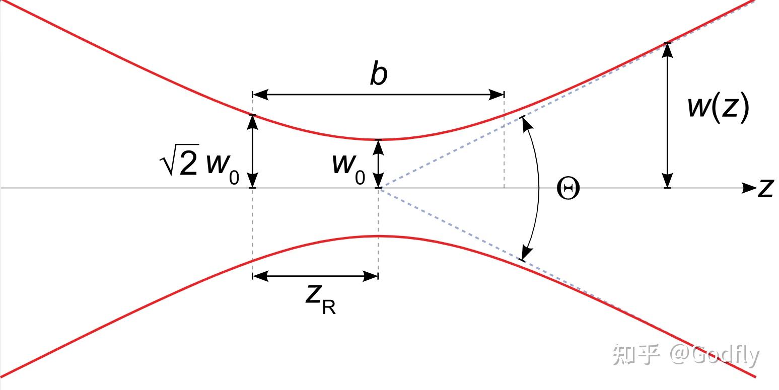
The beam waist width w0, Rayleigh length zR, and divergence angle theta of a Gaussian beam, image source: Wikipedia

The magnitude of the electric field strength of an ordinary Hermite-Gaussian beam is as follows:

\[\begin{aligned} E_{m,n}(x,y,z) = & \,E_0 \color{blue}{ \frac{w_0}{w(z)}\exp\left[-\frac{x^2+y^2}{w(z)^2}\right] } \times \\ & \color{green}{\exp\left[-\mathrm{i}\frac{k(x^2+y^2)}{2 R(z)}\right]} \color{orange}{\exp\left[\mathrm{i}\psi(z)\right]} \color{gray}{\exp[-\mathrm{i}kz]} \times \\ & \color{red}{H_m\left[\sqrt{2}\frac{x}{w(z)}\right]H_n\left[\sqrt{2}\frac{y}{w(z)}\right]} \end{aligned} \]

where:

\(\color{blue}{w(z) = w_0 \sqrt{1+\left(\frac{z}{z_R}\right)^2}}\) denotes the beam width at \(z\), and \(z_R = \pi\frac{w_0^2}{\lambda}\) is the Rayleigh length, defined as the value of \(z\) when the beam width has diverged to \(\sqrt{2}\) times the waist width.

\(\color{green}{R(z) = \frac{z^2 + z_R^2}{z}}\) denotes the radius of curvature of the wavefront at \(z\).

\(\color{orange}{\psi(z)=\arctan\left(\frac{z}{z_R}\right)}\) denotes the Gouy phase shift. From negative infinity to positive infinity, there is a total additional phase shift of \(\pi\).

\(\color{red}{H_m(t)}\) is the \(m\)-th order Hermite polynomial. They are also the energy eigenfunctions of the quantum harmonic oscillator. When \(m,n\) are both zero, this reduces to the fundamental Gaussian beam. Most lasers output fundamental Gaussian beams.

Clearly, Gaussian beams are not difficult to memorize: one only needs to remember three features: \(\color{blue}{\text{束腰发散}}\), \(\color{green}{\text{曲率半径}}\), and \(\color{orange}{\text{古伊相移}}\).

Another useful quantity is the divergence angle. From \(\color{blue}{w(z) = w_0 \sqrt{1+\left(\frac{z}{z_R}\right)^2}}\), one can see that the tangent of the divergence angle is \(\tan \theta=\frac{w_0}{z_R}\), and thus \(w_0 \tan \theta = \frac{\lambda}{\pi}\).

The shape of a Gaussian beam is completely determined by any two of the following three quantities: wavelength, beam waist radius, and divergence angle. The relation among these three is given by \(w_0 \tan \theta = \frac{\lambda}{\pi}\).

\(E_{m,n}(x,y,z)\) represents only the magnitude of the electric field strength and does not include polarization information.

Adding polarization information is easy: for polarization in the \(x\) direction, one only needs to multiply \(E_{m,n}(x,y,z)\) by the unit vector \(\hat{x}\) in the \(x\) direction. For circular polarization, simply multiply by \(\hat{x} \pm \mathrm{i}\hat{y}\).

Note that \(E_{m,n}(x,y,z)\) is a complex number. For classical electromagnetic waves, the actual electric field strength is its real part. For quantum electromagnetic waves, we can specify an annihilation operator for this mode; this annihilation operator is a linear combination of plane-wave annihilation operators, with coefficients obtainable through Fourier analysis.

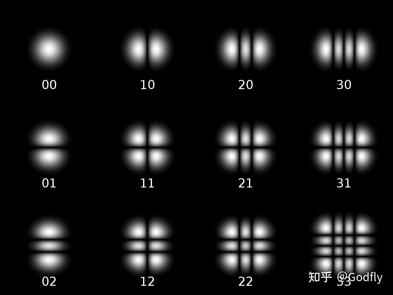
HG modes, image source: Wikipedia

II. Laguerre-Gaussian (LG) Beams

Among the solutions of the two-dimensional quantum harmonic oscillator, in addition to the linear oscillations represented by Hermite polynomials, there are rotational motions represented by Laguerre polynomials.

We now give the form of the Laguerre-Gaussian beam:

\[\begin{aligned} E_{l,p}(r,\varphi,z) = & \,E_0 \color{blue}{ \frac{w_0}{w(z)}\exp\left[-\frac{r^2}{w(z)^2}\right] } \times \\ & \color{green}{\exp\left[-\mathrm{i}\frac{kr^2}{2 R(z)}\right]} \color{orange}{\exp\left[\mathrm{i}\psi(z)\right]} \color{gray}{\exp[-\mathrm{i}kz]} \times \\ & \color{red}{\left(\sqrt{2}\frac{r}{w(z)}\right)^{|l|} L_p^{|l|} \left(2 \frac{r^2}{w(z)^2}\right) \exp(-\mathrm{i}l\varphi)} \end{aligned} \]

Here, \(\color{blue}{\text{束腰发散}}\) and \(\color{green}{\text{曲率半径}}\) are the same as for Hermite-Gaussian beams. There are two differences:

First, the higher-order terms change from Hermite polynomials to Laguerre polynomials \(\color{red}{L_p^{|l|} (t)}\). The additional factors \(\color{red}{\left(\sqrt{2}\frac{r}{w(z)}\right)^{|l|}}\) and \(\color{red}{\exp(-\mathrm{i}l\varphi)}\) represent, respectively, the singularity at the origin and the helical wavefront (carrying orbital angular momentum \(\hbar l\)).

Second, the Gouy phase shift \(\color{orange}{\psi(z) = (2p + |l|+ 1)\arctan \frac{z}{z_R}}\) becomes \(2p + |l|+ 1\) times that of the HG mode.

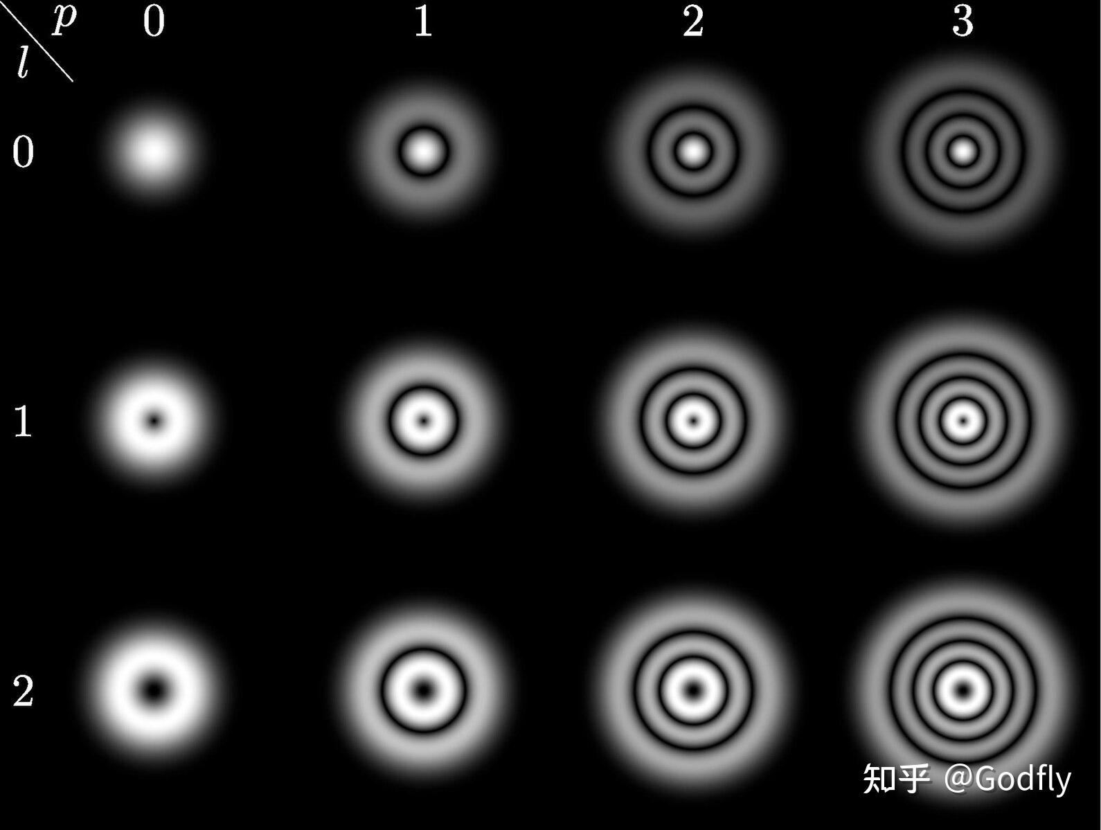
LG modes, image source: Wikipedia

Just as rotation can be decomposed into a linear superposition of oscillations, LG modes can also be expressed as coherent superpositions of HG modes. This is similar to how circular polarization can be decomposed into a superposition of two linear polarizations.

III. Manipulating Spin and Orbital Angular Momentum with Q-Plates

The q-plate proposed in 2006 [4] is essentially a half-wave plate whose optical axis depends on position, where the angle \(\alpha\) of the optical axis satisfies \(\alpha(r,\varphi) = q \varphi + \alpha_0\). Its Jones matrix is \(\begin{bmatrix} \cos 2\alpha & \sin 2\alpha \\ \sin 2\alpha & -\cos 2\alpha \end{bmatrix}\).

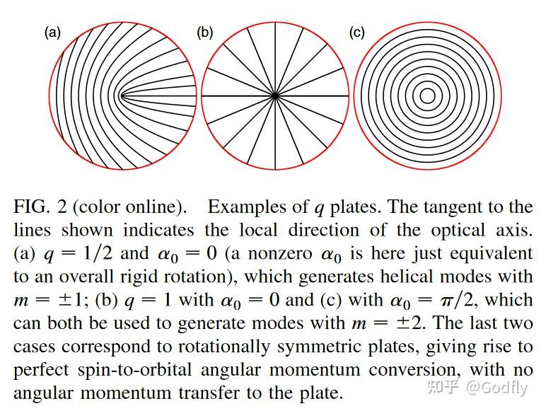
Optical-axis pattern of a q-plate, image source: [4]

Consider a q-plate acting on a fundamental Gaussian beam with left-circular polarization. The result is:

\[\begin{bmatrix} \cos 2\alpha & \sin 2\alpha \\ \sin 2\alpha & -\cos 2\alpha \end{bmatrix} \begin{bmatrix} \frac{1}{\sqrt{2}} \\ \frac{\mathrm{i}}{\sqrt{2}} \end{bmatrix} = e^{\mathrm{i}2q\varphi} \begin{bmatrix} \frac{1}{\sqrt{2}} \\ -\frac{\mathrm{i}}{\sqrt{2}} \end{bmatrix}\]

Clearly, after passing through the q-plate, left-circularly polarized light becomes right-circularly polarized light carrying orbital angular momentum \(2q\hbar\).

q-plates are currently the most commonly used method for experimentally preparing OAM states. Of course, an SLM can also be used.

One reason OAM attracts the interest of quantum information researchers is that, like the harmonic oscillator, its Hilbert-space dimension is infinite, unlike polarization (SAM), which has only two dimensions. The interaction between SAM and OAM suggests a straightforward idea: using SAM and OAM to construct a CNOT gate, where SAM is the control bit and OAM is the target bit. There are many similar experiments, so references will not be listed here.

References

1. ^Allen, L.; Beijersbergen, M. W.; Spreeuw, R. J. C.; Woerdman, J. P. Orbital Angular Momentum of Light and the Transformation of Laguerre-Gaussian Laser Modes. Phys. Rev. A 1992, 45 (11), 8185–8189. https://doi.org/10.1103/PhysRevA.45.8185.
2. ^A. Mair, A. Vaziri, G. Weihs, and A. Zeilinger, “Entanglement of the orbital angular momentum states of photons,” Nature 412(6844), 313–316 (2001).
3. ^Padgett, M. J. Orbital Angular Momentum 25 Years on [Invited]. Opt. Express 2017, 25 (10), 11265. https://doi.org/10.1364/OE.25.011265.
4. ^Marrucci, L.; Manzo, C.; Paparo, D. Optical Spin-to-Orbital Angular Momentum Conversion in Inhomogeneous Anisotropic Media. Phys. Rev. Lett. 2006, 96 (16), 163905. https://doi.org/10.1103/PhysRevLett.96.163905.