[Quantum Optics Experiment Notes · III] Quantum State Tomography

Quantum State Tomography

Quantum state tomography is the process of inferring a quantum state from the measurement results of an ensemble of quantum states. Its formulation is very simple, as follows:

Given a set of measurement operators \(\{\Pi_1,\cdots,\Pi_n\}\) and their corresponding measurement probabilities \(p_k=\operatorname{Tr}[\rho \Pi_k]\), find the quantum state \(\rho\).

In other words, in these n equations \(p_k=\operatorname{Tr}[\rho \Pi_k]\), \(p_k\) and \(\Pi_k\) are known, and \(\rho\) is to be found.

Conversely, if \(\rho\) and \(p_k\) are known and one seeks \(\Pi_k\), this is called detector tomography. However, that is not the subject of this article.

Why should we care about state tomography? Because we want to know exactly what the quantum states prepared experimentally look like. The method is state tomography.

It can be seen from the equation \(p_k=\operatorname{Tr}[\rho \Pi_k]\) that if \(\rho\) has \(n\) degrees of freedom, then we need at least \(n\) measurement operators, and these measurement operators must also be “mutually independent.” This condition is called tomographical completeness or informational completeness.

Why is it called “tomography”?
State tomography is called “tomography” because the tomography of continuous-variable photonic states is genuinely very similar to CT (computed tomography) performed in hospitals. In CT, projection images at various angles are known and a three-dimensional image is reconstructed; in the tomography of continuous-variable photonic states, projection images at various angles are known and a Wigner function is reconstructed. The latter is a kind of “two-dimensional image.”
Of course, it can also be understood using discrete variables, because (von Neumann) measurement is simply projection, while tomography reconstructs the original quantum state from the measured projections.
In short, tomography is called tomography because it is a process of reconstructing the whole from projections.

State Tomography of a Qubit

The density operator of a qubit has only three degrees of freedom (the Bloch vector), so theoretically only three measurement operators are needed. For example, one may choose the three measurement operators \(\{(\mathbb{I}+X)/2,\,\, (\mathbb{I}+Y)/2,\,\, (\mathbb{I}+Z)/2 \}\) (where \(X,Y,Z\) are the Pauli matrices). They correspond to the X, Y, and Z axes on the Bloch sphere, equivalent to measuring the x, y, and z components of the Bloch vector, respectively.

However, the problem is that experimentally, we do not measure probabilities directly; rather, we measure counts of outcomes. If we want to know the probability \(p_Z=\operatorname{Tr}[\rho (\mathbb{I}+Z)/2] = \langle0|\rho|0\rangle\), we must use the count \(p_Z=\frac{N_Z}{N_Z+N_{-Z}}\), while measuring \(N_{-Z}\) requires an additional measurement operator \((\mathbb{I}-Z)/2\).

More generally, because what we measure are counts and normalization is required, the actual number of measurement operators needed is always one more than theoretically required. The density operator of N qubits has \(4^n-1\) degrees of freedom, and adding one gives exactly \(4^n\).

For n=1, we therefore need 4 measurement operators. This is also the method used in the earliest article on photonic-state tomography[1].

Alright, enough chatter. Let us study the tomography of a qubit in detail, which will help with the later generalization to multiple qubits.

The density operator of a qubit is \(\rho = \frac{\mathbb{I}+xX+yY+zZ}{2}\), and performing tomography on it means solving for \(x, y,z\). As stated above, we choose four measurement operators: \(\{(\mathbb{I}+X)/2,\,\, (\mathbb{I}+Y)/2,\,\, (\mathbb{I}+Z)/2, \,\,(\mathbb{I}-Z)/2 \}\). The measured counts are then respectively

\[N_{X} = N p_X = N \operatorname{Tr}[\rho \frac{\mathbb{I}+X}{2}] = N\frac{1+x}{2}\]\[N_{Y} = N p_Y = N \operatorname{Tr}[\rho \frac{\mathbb{I}+Y}{2}] = N\frac{1+y}{2}\]\[N_{Z} = N p_Z = N \operatorname{Tr}[\rho \frac{\mathbb{I}+Z}{2}] = N\frac{1+z}{2}\]\[N_{-Z} = N p_{-Z} = N \operatorname{Tr}[\rho \frac{\mathbb{I}-Z}{2}] = N\frac{1-z}{2}\]

By solving these four equations simultaneously, we can obtain the four unknowns \(x,y,z,N\).

OK, that is it. It is that simple.

Maximum Likelihood Estimation

Wait, is it really that simple? Sharp-eyed readers may notice that a density operator is required to be positive definite, but no step in the solving procedure above can ensure positive definiteness.

In fact, if one solves the problem according to the above steps, it is entirely possible to obtain a density operator that is not positive definite. In other words, one obtains a “non-physical” result.

This is because experimental data contain errors, which in some cases lead to non-physical results.

Note that this is not error caused by an imperfect experimental system, but rather error inherent to quantum statistics itself, or fluctuation. For example, for a coherent state, its count distribution is Poissonian, with variance equal to the mean. When time is limited and a large amount of data cannot be acquired, the relative error \(\frac{\Delta N}{N}=\frac{1}{\sqrt{N}}\) can be relatively large.

Some readers may immediately say: then why not simply impose an additional constraint on the result? In this example, requiring \(|x|,|y|,|z|\le1\) is sufficient to guarantee positive definiteness.

But then another problem arises: after adding the constraint, cases that are not positive definite simply become unsolvable.

OK, since the lack of a solution is caused by errors, we can settle for the next best thing and turn the problem from an [equation-solving problem] into a [fitting problem].

What is a fitting problem? We know that two points determine a line. But when the data points themselves have large errors, we need many points, and these points will almost certainly not lie on the same line; in that case, the line equation has no solution.

Although there is no solution, we can fit it! We can use the least-squares method!

So where does the least-squares method come from? The answer is maximum likelihood estimation (MLE).

The idea of maximum likelihood estimation is to find a line such that, among all possible lines, it is the one most likely to have produced the points we measured. Specifically, one defines a likelihood function whose independent variables are the parameters of the line and whose value is the probability of measuring the observed results given that line. The entire problem then becomes an optimization problem: find the maximum of the likelihood function and the corresponding line parameters.

In many cases, experimental errors are assumed to follow a normal distribution. The likelihood function then has an exponential form \(L=e^{-\mathcal{L}}\). We then take the logarithm of the likelihood function and negate it to obtain a new likelihood function \(\mathcal{L}\), and find the minimum of the new likelihood function \(\mathcal{L}\). This new likelihood function can generally be interpreted as “the total error between the theoretically measured results and the actual measured results, assuming this line.”

All of the ideas above can be directly applied to state tomography. We can define a likelihood function whose independent variables are the degrees of freedom of the positive-definite matrix \(\rho\), and whose value is the probability of obtaining the observed results given that the quantum state is \(\rho\).

Below, we translate these ideas into an algorithm:

Define a valid density operator \(\rho(x,y,z)=\frac{\mathbb{I}+xX+yY+zZ}{2}, |x|,|y|,|z|\le1\)

Define the likelihood function as the probability of measuring the actual results under the assumption that the quantum state is \(\rho\):

\[\begin{aligned} \mathcal{L}(x,y,z) &= P(N_1=n_1,N_2=n_2,\cdots) \\ &= \prod_k \exp\left[-\frac{(n_k-\hat{n}_k)^2}{2\hat{n}_k}\right]\\ &= \prod_k \exp\left[-\frac{(n_k-N\operatorname{Tr}[\rho \Pi_k])^2}{2N\operatorname{Tr}[\rho \Pi_k]}\right] \end{aligned}\]

A continuous normal distribution is used here rather than a discrete Poisson distribution because when the count is large (experimentally, typically at least several hundred to several thousand), the normal distribution can approximate the Poisson distribution well.

The Poisson distribution may also be used as the likelihood function, but the result (see the appendix) is not as intuitive, and it is more computationally demanding.

For convenience of calculation, take the negative logarithm and remove unnecessary constants \(N\), obtaining:

\[\begin{aligned} \mathcal{L}(x,y,z)=\sum_k\frac{\left(p_k-\hat{p}_k\right)^2}{2\hat{p}_k}=\sum_k\frac{\left(p_k-\operatorname{Tr}[\rho(x,y,z)\Pi_k]\right)^2}{2\operatorname{Tr}[\rho(x,y,z)\Pi_k]} \end{aligned}\]

At this point, we need only solve \((x_0,y_0,z_0) = \underset{|x|,|y|,|z|\le1}{\operatorname{arg\,min}} \mathcal{L}(x,y,z)\).

This is a constrained optimization problem. Can it be transformed into an unconstrained optimization problem? See below.

State Tomography of Multiple Qubits

The density operator of n qubits has \(4^n -1\) degrees of freedom. The counterpart of the Bloch vector in this case is the Pauli correlator:

\[\begin{aligned} \rho = \frac{1}{2^n}\sum_{i_1,\cdots,i_n=0}^{3} c_{i_1i_2\cdots i_n} \sigma_{i_1} \otimes \sigma_{i_2} \otimes \cdots \sigma_{i_n} \end{aligned}\]

Here, \(\sigma_i,\,i=0,1,2,3\) are respectively the identity matrix and the Pauli matrices \(\mathbb{I},X,Y,Z\). Moreover, \(c_{i_1i_2\cdots i_n}\) are called correlators.

At this point, we need at least \(4^n\) measurement operators. After measuring counts under these operators, we can perform maximum likelihood estimation.

The state \(\rho\) can now be set to \(\rho(\mathbf{t})=\frac{T^\dag(\mathbf{t})T(\mathbf{t})}{\operatorname{Tr}(T^\dag(\mathbf{t})T(\mathbf{t}))}\), where

\[T(\mathbf{t})=\begin{bmatrix} t_1 & 0 & 0 & \cdots & 0 \\ t_{2^n+1}+it_{2^n+2} & t_2 & 0 & \cdots & 0 \\ t_{2^n+5}+it_{2^n+6} & t_{2^n+3}+it_{2^n+4} & t_3 & \cdots & 0 \\ \vdots & \vdots & \vdots & \ddots & \vdots \\ t_{4^n - 1}+it_{4^n} & t_{4^n - 3}+it_{4^n-2} & t_{4^n - 5}+it_{4^n-4} & \cdots & t_{2^n} \end{bmatrix}\]

This is to ensure the positive definiteness of \(\rho(\mathbf{t})\).

Compared with using the correlators \(c_{i_1i_2\cdots i_n}\) as parameters and constraining their absolute values to be no greater than one, the advantage of this T(t) parameterization is that it transforms the maximum likelihood estimation to be performed into an unconstrained problem (we impose no constraints on t).

The likelihood function is then:

\[\begin{aligned} \mathcal{L}(\mathbf{t})=\sum_k\frac{\left(p_k-\hat{p}_k\right)^2}{2\hat{p}_k}=\sum_k\frac{\left(p_k-\operatorname{Tr}[\rho(\mathbf{t})\Pi_k]\right)^2}{2\operatorname{Tr}[\rho(\mathbf{t})\Pi_k]} \end{aligned}\]

Choosing Measurement Operators

What kinds of measurement operators are best to choose?

For polarization-encoded photonic qubits, we generally simply use the six projective measurements H, V, D, A, R, and L, together with their combinations (they are easy to implement, requiring only wave plates). For n qubits, we then have \(6^n\gt 4^n\) projection operators, which is sufficient.

Since \((|H\rangle\langle H|, |V\rangle\langle V|)\) constitute a POVM, \((|D\rangle\langle D|, |A\rangle\langle A|)\) constitute a POVM, and \((|R\rangle\langle R|, |L\rangle\langle L|)\) constitute a POVM, that is, six projective measurements correspond to three POVMs, we need \(3^n\) POVMs, which experimentally means \(3^n\) measurement settings (a measurement setting refers to the angles of the wave plates).

But then the question arises: is there a better way to reduce the number of POVMs, thereby reducing the time required for tomography? After all, \(6^n\gt 4^n\) is redundant.

From this point onward, this can be considered a frontier problem in academia, and I could promote some work from our group. I will write about it when I have time in the future, haha.

State Tomography of Continuous-Variable Photonic States

So-called continuous-variable photonic states are those that consider the entire Fock Space, rather than only the subspace of zero- and one-photon states within the Fock Space. We care about continuous variables because a photon is fundamentally a harmonic-oscillator system rather than a two-level system. Considering the former is more natural and more consistent with the nature of photons. In fact, the classical electromagnetic waves encountered in daily life are continuous-variable photonic states (namely coherent states).

Single-mode continuous-variable photonic states can be described by quasiprobability distribution functions. There are three quasiprobability distribution functions: the Glauber P-, Husimi Q-, and Wigner functions, abbreviated as the P-, Q-, and W- representations, respectively. Since only the marginal distributions of the Wigner function correspond to the probability distributions of actual observables, we generally consider the Wigner function.

What is the Wigner function?

How should one understand the Wigner function? We can begin with classical electromagnetic waves. We all know that a single-mode (single-frequency) electromagnetic wave can be described by a point in the complex plane (that is, by a phase-space diagram). The superposition of electromagnetic waves directly corresponds to complex-number addition (or vector addition) in phase space.

This so-called phase-space representation can immediately be extended to quantum mechanics. For a quantized single-mode classical electromagnetic field, its phase-space representation is no longer an infinitesimal point, but a circle of finite size. In fact, it is a Gaussian function on the complex plane, and the standard deviation of this Gaussian function is determined by the uncertainty principle. This Gaussian function is the Wigner function of a classical electromagnetic wave, and its marginal distributions correspond to the probability distributions of the electric-field strength of that quadrature (the electric field is also an observable and has uncertainty). The quantum state obtained after quantizing a classical electromagnetic wave is called a coherent state.

For a more general quantum optical field, its Wigner function can take all sorts of strange shapes and may even have negative values. Of course, this does not mean that we obtain negative probabilities—after taking marginal distributions, we always obtain nonnegative probabilities. This is because the areas occupied by these negative values are sufficiently small that they are smaller than the area allowed by the uncertainty principle; in other words, the uncertainty principle ensures that we cannot observe negative probabilities.

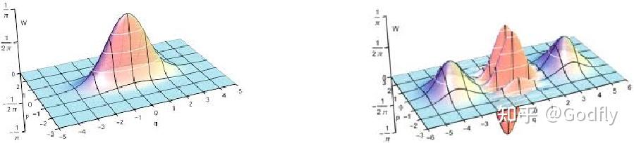
Wigner functions of several interesting photonic states. The left image shows a squeezed state, and the right image shows a Schrödinger cat state.

State tomography of continuous-variable photonic states is performed by measuring quadratures. In this case, all measurement operators have the following form:

\[\begin{aligned} \Pi_\theta = \frac{ae^{-i\theta}+a^\dag e^{i\theta}}{2} \end{aligned}\]

This is the so-called “quadrature” (I do not know its Chinese translation). Intuitively, it projects the entire Wigner function onto a line, where the angle between this line and the x-axis is \(\theta\).

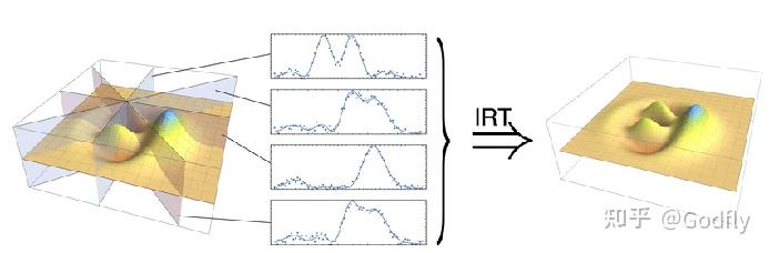
Quantum state tomography of continuous-variable optical states

Quantum information theory tells us that if we wish to reconstruct the Wigner function (with infinite precision), we need infinitely many \(\theta\), that is, countless measurement operators. Of course, we do not need infinite precision, so we only need to choose \(\theta\) sufficiently densely. For example, using a step size of 0.01 radians, from 0 to 2pi.

After obtaining the probability density distributions of the quadratures, we can use the inverse Radon transform to reconstruct the Wigner function. This is exactly the same principle as CT in hospitals.

As for how to measure quadratures experimentally, it is very simple: as in radio, one only needs to mix the signal with a local oscillator. This is called homodyne measurement. Specifically, the signal to be measured and a laser are mixed using a beam splitter, and the difference between the two output signals is recorded. Changing the phase of the laser changes \(\theta\).

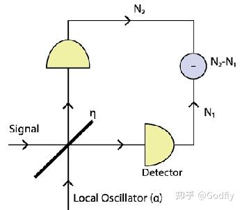
Homodyne Measurement

Appendix: Maximum Likelihood Estimation for the Poisson Distribution

The likelihood function corresponding to the Poisson distribution is

\[ \begin{aligned} \mathcal{L}(\mathbf{t}) &= P(N_1=n_1,N_2=n_2,\cdots) \\ &= \prod_k e^{-\lambda_k} \frac{\lambda_k^{n_k}}{n_k!} \\ &\xrightarrow{-\log} \sum_k (\lambda_k - n_k \log \lambda_k + \cancel{\log n_k!}) \\ &\xrightarrow{\frac{1}{N}} \sum_k(\hat{p}_k(\mathbf{t})-p_k \log \hat{p}_k(\mathbf{t})) \end{aligned}\]

where \(\lambda_k = N \operatorname{Tr}[\rho(\mathbf{t}) \Pi_k]= N \hat{p}_k(\mathbf{t})\).

Taking the derivative of the likelihood function and finding its minimum reveals that the minimum is attained when \(\hat{p}_k(\mathbf{t}) = p_k\). This shows that using the Poisson distribution is also correct. However, the likelihood function for the Poisson distribution contains logarithms, whereas the likelihood function for the normal distribution contains only polynomials. The latter is more computer-friendly and converges somewhat faster. Therefore, we generally use the likelihood function corresponding to the normal distribution.

References

1. ^James, D. F. V., Kwiat, P. G., Munro, W. J. & White, A. G. Measurement of qubits. Phys. Rev. A 64, 052312 (2001).