[Quantum Optics Experimental Notes I] Principles of Measuring the Second-Order Correlation Function (g2) with Single-Photon Detectors

HBT Experiment

Anyone doing quantum optics experiments certainly knows that the HBT experiment can be used to measure the second-order correlation function g2. That is, a beam of light is split into two beams using a 50:50 beam splitter, which are then detected by two separate detectors, and the variation of the correlation between the intensities on the two sides with delay is counted, as shown below:

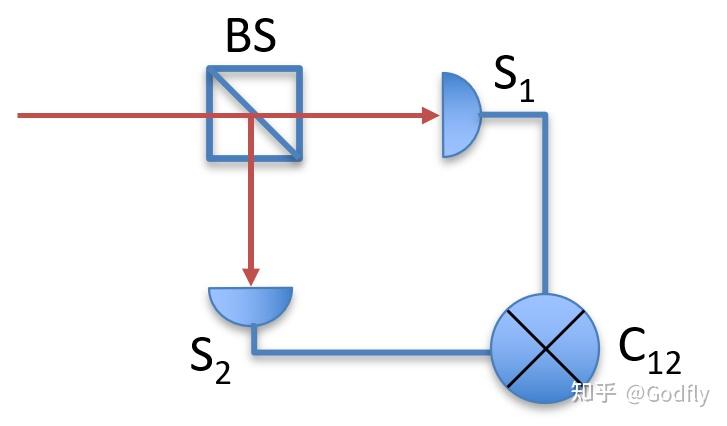
Hanbury Brown and Twiss Experiment

The classical normalized g2 is defined as

\[\begin{aligned} g^{(2)}(r_1,r_2;\tau)&=\frac{\langle E^*(r_1,t)E^*(r_2,t+\tau) E(r_2,t+\tau)E(r_1,t)\rangle}{\langle |E(r_1,t)|^2\rangle\langle |E(r_2,t+\tau)|^2\rangle} \\ &= \frac{\langle I(r_1,t)I(r_2,t+\tau)\rangle}{\langle I(r_1,t)\rangle\langle I(r_2,t+\tau)\rangle} \end{aligned}\]

where \(E\) denotes the electric field, and \(I\) denotes the light intensity. Clearly, according to the definition, what the HBT experiment measures is the classical g2 (simply divide the correlated light intensity by the product of the individual intensities on the two sides).

Quantum Second-Order Optical Correlation Function

The quantum normalized g2 is defined as:

\[\begin{aligned} g^{(2)}(r_1,r_2;\tau)&=\frac{\langle E^-(r_1,t)E^-(r_2,t+\tau) E^+(r_2,t+\tau)E^+(r_1,t)\rangle}{\langle E^-(r_1,t)E^+(r_1,t)\rangle\langle E^-(r_2,t+\tau)E^+(r_2,t+\tau)\rangle} \end{aligned}\]

Comment: In the quantum case, the operators in the numerator must be replaced by the negative-frequency component \(E^-\) and the positive-frequency component \(E^+\) of the electric field, which respectively contain creation and annihilation operators.
Moreover, the creation operators must come before the annihilation operators, because detecting a photon is an annihilation process, unlike in the classical case. The coherent state \(|\alpha\rangle\) in the classical case is an eigenstate of the annihilation operator \(a|\alpha\rangle=\alpha|\alpha\rangle\) ; adding or removing one photon makes no difference.

In the single-mode case, since \(E^+=i\sqrt{\frac{\hbar \omega}{2\epsilon_0 V}}a\) and \(E^-=i\sqrt{\frac{\hbar \omega}{2\epsilon_0 V}}a^\dag\) , the quantum g2 can be simplified to

\[\begin{aligned} g^{(2)}(r_1,r_2,\tau)&=\frac{\langle a^\dag(r_1,t)a^\dag(r_2,t+\tau)a(r_2,t+\tau)a(r_1,t)\rangle}{\langle n(r_1,t)\rangle\langle n(r_2,t+\tau) \rangle} \end{aligned}\]

Therefore, to measure quantum g2, we need to replace the intensity detector with a photon detector, and this photon detector must be able to resolve photon number.

However, here comes the problem: currently available photon-number-resolving single-photon detectors are all rather unsatisfactory. TES has an excessively long recovery time; spatial and temporal demultiplexing schemes provide only pseudo photon-number resolution; and SNSPDs are expensive, require cryogenic temperatures, and may not have particularly high multiphoton efficiency.

Measuring g2 with NPNR-SPDs

Fortunately, single-photon detectors that cannot resolve photon number (NPNR-SPDs, Non-Photon-Number-Resolving Single-Photon Detectors) can also measure g2, even though they cannot resolve photon number!

Comment: “Unable to resolve photon number” means that they can distinguish only between “no photon” and “one or more photons.” Common APD detectors cannot resolve photon number.

The method is simple: just make the quantum efficiency of the NPNR-SPD sufficiently low!

The so-called quantum efficiency \(\eta\) is the probability that the detector can detect a photon, given that one photon enters the detector. Conversely, the probability that this photon is “lost” is \(1-\eta\) .

At first, I found this strange: how could lower efficiency be better? But with a little thought, the principle becomes clear:

When the efficiency is sufficiently low, the probability that \(k\) photons are not all lost is \(1-(1-\eta)^k\approx k\eta\) . In other words, the probability that an NPNR-SPD detects photons is proportional to \(k\) . In this way, we effectively achieve “photon-number resolution” through “low efficiency.”

The formal (boring) mathematical derivation follows; you may skip it:
Let the count rate of detector 1 be \(S_1\) , the count rate of detector 2 be \(S_2\) , the coincidence count rate (detecting photons simultaneously) of the two detectors be \(C_{12}\) , and the number of photons in the beam per unit time be \(R\) . Then:
\(\begin{aligned} S_i &=R\sum_{n=1}^{\infty}\frac{P_n}{2^n}\sum_{k=1}^{n}C_n^k[1-(1-\eta)^k] \\ &\approx R \sum_{n=1}^{\infty}\frac{P_n}{2^n}\sum_{k=1}^{n}C_n^k\cdot k\eta \\ &= R\frac{\eta}{2} \sum_{n=1}^{\infty} n P_n \end{aligned}\)
\(\begin{aligned} C_{12}&=R\sum_{n=1}^{\infty}\frac{P_n}{2^n}\sum_{k=1}^{n-1} C_n^k[1-(1-\eta)^k][1-(1-\eta)^{(n-k)}] \\ &\approx R \sum_{n=1}^{\infty}\frac{P_n}{2^n}\sum_{k=1}^{n}C_n^k\cdot k\eta \cdot (n-k)\eta \\ &= R \frac{\eta^2}{4} \sum_{n=2}^{\infty} n(n-1)P_n \end{aligned}\)
Thus
\(\begin{aligned} \frac{C_{12} R}{S_1 S_2} &= \frac{\sum_{n=2}^{\infty} n(n-1)P_n }{\left(\sum_{n=1}^{\infty} n P_n\right)^2} \\ &= \frac{\langle n(n-1) \rangle}{\langle n\rangle^2} \end{aligned}\)
Those familiar with quantum optics should already recognize that this is g2. The derivation is as follows:
\(\begin{aligned} g^{(2)}(r_1,r_2,\tau)&=\frac{\langle a^\dag(r_1,0)a^\dag(r_2,\tau)a(r_2,\tau)a(r_1,0)\rangle}{\langle n(r_1)\rangle\langle n(r_2) \rangle} \end{aligned}\)
Setting \(r_1=r_2,\quad \tau=0\) gives
\(\begin{aligned} g^{(2)}(\tau=0)&=\frac{\langle a^\dag a^\dag a a \rangle}{\langle n\rangle^2} \\ &= \frac{\langle a^\dag(aa^\dag -1) a\rangle}{\langle n\rangle^2} \\ &= \frac{\langle n^2-n\rangle}{\langle n\rangle^2} \end{aligned}\)

What is the use of measuring g2? Besides the textbook applications of distinguishing [super-Poissonian statistics/Poissonian statistics/sub-Poissonian statistics] and [photon bunching/antibunching], it has another unexpected application: measuring the spectral correlations of photons. We will discuss this in the next article.

Epilogue: The Multimode Case

Earlier, we planted a small foreshadowing: we assumed that the detected light was single-mode. Thus \(E^+\) can be proportional to \(a\) : \(E^+=i\sqrt{\frac{\hbar \omega}{2\epsilon_0 V}}a\) .

But what happens if the detected light is multimode? In this case, \(E^+=i\sum_{k}\sqrt{\frac{\hbar \omega_k}{2\epsilon_0 V}}a_k\) , and \(E^+\) is no longer proportional to \(a\) ; instead, it has a frequency dependence: \(E^+_k\propto \sqrt{\omega_k}a_k\) .

Since the original g2 detects light intensity, and light intensity equals frequency multiplied by photon number, it is not surprising that there is a term \(\sqrt{\omega_k}\) here.

However, as long as the frequencies of the various modes are the same, we can still cancel \(\sqrt{\omega_k}\) and obtain:

\[\begin{aligned} g^{(2)}(0)=\frac{\left\langle :\left(\sum_k a^\dag_k a_k\right)^2:\right\rangle}{\left\langle \sum_k a^\dag_k a_k\right\rangle^2} \end{aligned}\]

where \(::\) denotes normal ordering, i.e., moving all creation operators before the annihilation operators.

Setting \(n=\sum_ka^\dag_k a_k\) , we have

\[\begin{aligned} g^{(2)}(0)=\frac{\langle n(n-1)\rangle}{\langle n\rangle^2} \end{aligned}\]

It can be seen that although multiple modes are present, if the frequencies of these modes are the same (approximately), then the HBT method for measuring quantum g2 remains valid.