An Introduction to Differential Geometry (Physics Version)

Preface

As a physics student, you have probably heard of one or more of the concepts tensor, differential form, exterior algebra, connection/curvature, and so on. But, like me, you may feel completely lost whenever you hear these concepts. This article therefore aims to help physics students organize these closely interconnected ideas.

The structure of this article is as follows:

a. In Chapter 1, we introduce the stage on which physics takes place: differentiable manifolds, and define scalar fields on manifolds.

b. In Chapter 2, we define tangent vector fields, cotangent vector fields, and tensor fields on manifolds. We also define inner products and metric tensors, which are additional structures on manifolds.

c. In Chapter 3, we introduce concepts such as exterior products and exterior algebra, and study exterior differentiation on manifolds. Finally, we introduce the Hodge dual.

d. In Chapter 4, we introduce two kinds of derivatives: the covariant derivative and the Lie derivative.

The covariant derivative describes connections on manifolds and can be used to define parallel transport, geodesics, and curvature. Based on these concepts, we can give a brief introduction to general relativity;

The Lie derivative describes the “flow” of vector fields on manifolds. It is highly useful and can be used to define concepts such as divergence, torsion, and curvature concisely. It also leads to Lie algebras and Lie groups, but those are topics for another time and will not be covered here.

e. In Chapter 5, we introduce concepts such as simplices and chains, and study integration on manifolds. In addition, we briefly introduce homology and cohomology, which are used to study “holes” in manifolds.

Here are some statements and notes about this article:

a. Disclaimer

This article is merely my notes. I write with an imagined audience in mind, which may not only help others but also deepen my own understanding. However, precisely because this is only a set of notes, errors are inevitable. If readers find any factual errors, please point them out promptly. I will correct them as soon as possible to avoid misleading others.

This article mainly refers to Differential Geometry and Lie Groups for Physicists by Marián Fecko.

b. Intended Audience

The prerequisites for this article are elementary calculus and elementary linear algebra.

It is best suited to physics students. This article is suitable for second-year undergraduate physics students and above.

Mathematics students are also very welcome to read it, offer comments, and point out errors.

Rigor and accessibility are always opposing yet complementary. For the sake of accessibility, this article inevitably sacrifices some rigor in its wording. I therefore ask mathematics readers for their understanding.

c. Reading Suggestions

This article is intended to organize concepts, and should not be read as a tutorial. Of course, if you are simply interested, there is certainly no harm in reading it.

Chapter 1: Manifolds and Scalar Fields on Manifolds

This chapter introduces differentiable manifolds and the prerequisite concepts involved. Specifically, it first introduces topological spaces, then topological manifolds, and finally differentiable manifolds and scalar fields on them. Each concept is built on the preceding one.

1.1 Topology

A topology on a nonempty set \(X\) is defined as a collection \(\mathcal{F}\) of subsets of \(X\), where \(\mathcal{F}\) satisfies the following three properties:

a. \(\emptyset，X \in \mathcal{F}\) ；

b. The intersection of finitely many elements of \(\mathcal{F}\) is still in \(\mathcal{F}\);

c. The union of arbitrarily many elements of \(\mathcal{F}\) is still in \(\mathcal{F}\).

Comment

I am the first “comment” in this text. Here, “comment” refers to an interpretation and supplement to a concept. Let us now examine the concept of topology.

A topology is a collection \(\mathcal{F}\), whose elements are certain subsets of another set \(X\). Of course, these subsets are not chosen arbitrarily from \(X\); they must satisfy certain conditions. Specifically, they must be closed under finite intersections and arbitrary unions. In addition, the empty set and \(X\) itself are required to belong to the topology.

Let us look at some examples below.

Example 1.1
\(\{\emptyset,\{1,2,3\}\}\) is a topology on the set \(\{1,2,3\}\).
\(\{\emptyset,\{1,2,3\},\{1\}\}\) is a topology on the set \(\{1,2,3\}\).
\(\{\emptyset,\{1,2,3\},\{1\},\{2\},\{1,2\}\}\) is a topology on the set \(\{1,2,3\}\).
\(\{\emptyset,\{1,2,3\},\{1\},\{2\},\{3\},\{1,2\},\{1,3\},\{2,3\}\}\) is a topology on the set \(\{1,2,3\}\).

Example 1.2
All open sets in the Euclidean space \(\mathbb{R}^n\) form a topology on it.

1.2 Topological Spaces

A set equipped with a topology is called a topological space. More specifically, a topological space is defined as \((X,\mathcal{F})\), where \(\mathcal{F}\) is a topology on \(X\).

The elements of a topology are called open sets in the topological space.

Commentary

In a typical calculus course, we first define a metric on \(\mathbb{R}^n\), thereby making it a Euclidean space, and then define open sets through that metric.

The concept of topology allows us to define open sets without relying on a metric. In topology, we abstract the properties of “finite intersections” and “arbitrary unions” possessed by open sets in analysis, and use them to define open sets themselves.

If the context permits, we may simply call \(X\) a topological space, without explicitly writing \((X,\mathcal{F})\).

Optional Reading 1.2

You may wonder: why do we not define closed sets using “countable intersections” and “finite unions,” and then define topology from them? Why choose open sets rather than closed sets? This may involve various historical factors; see this question.

1.3 Continuity

Let \((X,\mathcal{F})\) and \((Y,\mathcal{S})\) be topological spaces, and let \(f:X\rightarrow Y\) be a map. If, for every \(\forall O \in \mathcal{S}\), we have \(f^{-1}[O] \in \mathcal{F}\), then \(f\) is called continuous. Here, \(f^{-1}[O]\) denotes the inverse image (preimage) of \(O\) under \(f\).

Commentary

Continuity means that “the inverse image of an open set is still open.” This is quite different from the definition of continuity in analysis.

The inverse image \(f^{-1}[O]\) of a set \(O\in Y\) under a map \(f:X\rightarrow Y\) is defined by:
\(f^{-1}[O]=\{x\in X\mid f(x)\in O \}\)

In mathematics, inverse images are generally denoted using parentheses \(f^{-1}(O)\), but in this article, to distinguish them from inverse maps, we use square brackets: \(f^{-1}[O]\).

Example 1.3

Under the topology in Example 1.2, the map \(f:\mathbb{R}\rightarrow\mathbb{R},\,f(x)=\begin{cases}1, & x\gt 0 \\ 0, & x=0\\ -1, & x\lt 0\end{cases}\) is not continuous, because the inverse image of the open set \(\{x\in \mathbb{R}\mid -1\lt x\lt 1\}\) under \(f\) is \(\{0\}\), which is not an open set.

1.4 Homeomorphism

If \(f:X\rightarrow Y\) is a bijection, and both \(f\) and its inverse are continuous, then \(f\) is called a homeomorphism from \(X\) to \(Y\).

If there is a homeomorphism from \(X\) to \(Y\), then we may also say that \(X\) and \(Y\) are homeomorphic.

Commentary

When we say that a coffee cup (with a handle) and a doughnut are homeomorphic, what we mean is that a one-to-one correspondence—a bijection—can be established between their points, and that this bijection is bicontinuous.

Nothing prevents you from establishing a bijection between a (spherical) piece of candy and a doughnut. But one thing is certain: such a bijection cannot be bicontinuous. In other words, a doughnut is not homeomorphic to a piece of candy.

1.5 Neighborhoods

Let \(X\) be a topological space, with \(p \in X\) and \(p \in O \subseteq N \subseteq X\), where \(O\) is an open set. Then \(N\) is called a neighborhood of \(p\).

Comment

Note that a neighborhood itself need not be an open set. If a neighborhood is open, it may be called an open neighborhood.

Of course, some authors define neighborhoods to be open neighborhoods; this depends on which book you are reading. In mathematics, the same concept may have many different definitions. This is fine—the key is to remain consistent within a given context.

1.6 Hausdorff Spaces

If, for any two elements \(x,y\) of a topological space \(X\), one can find a neighborhood \(U\) of \(x\) and a neighborhood \(V\) of \(y\) such that \(U\cap V=\emptyset\), then \(X\) is called a Hausdorff space.

Comment

Mathematicians may construct all sorts of strange non-Hausdorff spaces, but for us physicists, Hausdorff spaces are simply taken for granted. The manifolds introduced later are, by definition, all Hausdorff spaces.

1.7 Topological Manifolds

Let the Hausdorff topological space \(M\) have a countable open cover \(M=\bigcup_\alpha O_\alpha\) (\(O_\alpha\) is open), and suppose that every \(O_\alpha\) is homeomorphic to an open subset of \(\mathbb{R}^n\) (where \(\mathbb{R}^n\) carries the Euclidean topology familiar from elementary calculus). Then \(M\) is called an \(n\)-dimensional topological manifold.

Comment

Put simply, if every local part of \(M\) is homeomorphic to an open subset of \(\mathbb{R}^n\) (in the Euclidean sense), then \(M\) is called a topological manifold.

The “topology in the Euclidean sense” here refers to the point-set topology defined using the Euclidean metric, as covered in elementary calculus courses. Since this text assumes that readers have studied elementary calculus, we will not elaborate further.

A topological manifold looks locally like \(\mathbb{R}^n\), but globally it may differ greatly from \(\mathbb{R}^{n}\). For example, the surface of a “doughnut” locally looks like \(\mathbb{R}^2\), but globally it is completely different from \(\mathbb{R}^2\).

Topological manifolds are introduced because we want to assign coordinates to every point above.

For every point \(p \in O_\alpha\) on a topological manifold, there is a homeomorphism \(\varphi_\alpha: O_\alpha \rightarrow \varphi_\alpha[O_\alpha] \subseteq \mathbb{R}^n\) that assigns it coordinates.

However, one coordinate system is often insufficient; we need multiple coordinate systems \((O_\alpha,\varphi_\alpha)\) to cover the entire topological space.

Points in the overlap \(O_\alpha \cap O_\beta \) of the open cover have two sets of coordinates. The map \(\varphi_\beta\circ\varphi_\alpha^{-1}:\varphi_\alpha[O_\alpha \cap O_\beta]\rightarrow \varphi_\beta[O_\alpha \cap O_\beta]\) can be used to transform between these two coordinate systems.

This collection of open sets \(O_\alpha\) and their corresponding homeomorphisms \(\varphi_\alpha\) is called an atlas. More specifically, an atlas is defined as the set of all coordinate systems \((O_\alpha,\varphi_\alpha)\).

Comment

In many books, the direction of \(\varphi_\alpha\) is from an open subset of \(\mathbb{R}^n\) to the manifold \(M\), namely \(\varphi_\alpha:V_\alpha\subseteq \mathbb{R}^n\rightarrow M\), which is opposite to the direction defined above. In that case, the coordinate transformation is written as \(\varphi_\beta^{-1}\circ\varphi_\alpha\) rather than \(\varphi_\beta\circ\varphi_\alpha^{-1}\). However, since \(\varphi\) is a bijection, its direction is unimportant. Readers can determine the direction from the context.

1.8 Differentiable Manifolds

Denote the homeomorphism from an open set of the topological manifold \(M\) to an open subset of \(\mathbb{R}^n\) by \(\varphi_\alpha:O_\alpha\rightarrow \varphi_\alpha[O_\alpha]\subseteq \mathbb{R}^n\).

If, for every pair \(O_\alpha \cap O_\beta \neq \emptyset\), \(\varphi_\beta\circ\varphi_\alpha^{-1}\) is a smooth (infinitely differentiable) function, then the topological space \(M\) is called a differentiable manifold.

Comment

Since the coordinate transformation map \(\varphi_\beta\circ\varphi_\alpha^{-1}\) is smooth (infinitely differentiable), it ensures that the differentiable structure is not destroyed under coordinate transformations. See Section 1.9 for details.

Comment

A differentiable manifold may simply be called a manifold. When we speak of a manifold, we usually mean a differentiable manifold rather than a topological manifold.

You may wonder how the smoothness of \(\varphi_\beta\circ\varphi_\alpha^{-1}\) is defined. Note that \(\varphi_\beta\circ\varphi_\alpha^{-1}\) is merely a bijection between an open subset \(V_\alpha\) of \(\mathbb{R}^n\) and another open subset \(V_\beta\). Its differentiability was thoroughly discussed in elementary calculus, so there is no need to elaborate here.

In Section 1.3, we defined the continuity of maps (\(f:X\rightarrow Y\)) from topological spaces to topological spaces; this definition also applies to topological manifolds. However, we have not yet defined the smoothness of maps from differentiable manifolds to differentiable manifolds, namely the smoothness of \(f:M\rightarrow N\).

We can now define the smoothness of \(f:M\rightarrow N\). This definition requires \(\mathbb{R}^n\) as an intermediary, namely:

If \(\varphi_\beta\circ f \circ \varphi_\alpha^{-1}\) is smooth, then \(f\) is called smooth.

Likewise, note that \(\varphi_\beta\circ f \circ \varphi_\alpha^{-1}\) is a map from an open subset \(V_\alpha\) of \(\mathbb{R}^n\) to another open subset \(V_\beta\). Its differentiability was also thoroughly discussed in elementary calculus, so there is no need to elaborate here.

If \(f:M\rightarrow N\) is a smooth bijection, then \(f\) is called a diffeomorphism. Equivalently, \(M\) and \(N\) are said to be diffeomorphic.

1.9 Scalar Fields

Define a (real) scalar field \(f:M\rightarrow \mathbb{R}\) on a differentiable manifold as the composition of two maps: \(f=F\circ \varphi\).

Here, \(\varphi\) is a homeomorphism from \(O\) to \(\varphi[O]\subseteq \mathbb{R}^n\), and \(F\) is a function from \(\varphi[O]\) to \(\mathbb{R}\).

If \(F\) is also a smooth function from \(\varphi[O]\) to \(\mathbb{R}\), then \(f\) is called a smooth scalar field.

The set of all smooth scalar fields on \(M\) is denoted by \(\mathcal{F}(M)\).

Comment

To ensure that our smooth scalar fields are well-defined, we must ensure that there are no issues on the intersections of \(O_\alpha\) and \(O_\beta\). Fortunately, the smoothness of \(\varphi_\beta\circ\varphi_\alpha^{-1}\) guarantees this.

More specifically, on the intersection of \(O_\alpha\) and \(O_\beta\), we have
\(f=F_\alpha \circ \varphi_\alpha=F_\beta \circ \varphi_\beta \implies F_\alpha=F_\beta\circ \varphi_\beta \circ \varphi_\alpha^{-1}\).

If \(\varphi_\beta\circ\varphi_\alpha^{-1}\) were not a smooth function, then the smoothness of \(F_\beta\) would not guarantee the smoothness of \(F_\alpha\). This would make the definition ill-defined.

This is what is commonly called a “differentiable structure”: coordinate transformations do not alter the differentiability of functions.

Summary

In this chapter, we defined differentiable manifolds and scalar fields on manifolds. The steps are as follows:

First, we define a topology on a set to be the set of all its open subsets. Once a topology has been defined, the set is no longer merely a set, but a topological space.

Second, we wish to assign coordinates to every point in a topological space. This leads to a topological manifold, which locally looks like \(\mathbb{R}^n\) but globally differs from \(\mathbb{R}^n\). Specifically, we make each open set representing a “local” part of the topological space homeomorphic to an open subset of \(\mathbb{R}^n\), and then take the union of these open sets to cover the entire topological space. This characterizes a topological manifold.

Finally, we wish to study differentiation on topological manifolds, which leads to differentiable manifolds. A differentiable manifold is a topological manifold equipped with a differentiable structure; this structure ensures that smooth (infinitely differentiable) scalar fields on the differentiable manifold are well-defined. Specifically, it requires the coordinate transformation map \(\varphi_\beta\circ\varphi_\alpha^{-1}\) to be smooth, thereby ensuring that coordinate transformations do not destroy the smoothness of smooth scalar fields.

Chapter 2 Vector Fields and Tensor Fields on Manifolds

In this chapter, we first introduce concepts such as tangent spaces and dual spaces.

Next, based on these concepts, we define vector fields and tensor fields on differentiable manifolds.

Finally, we introduce inner products and metric tensors, which are additional structures on differentiable manifolds. Once equipped with a metric tensor, a differentiable manifold becomes a (pseudo-)Riemannian manifold.

2.1 Tangent Vectors and Tangent Spaces

Let \(\mathcal{F}(M)\) denote the set of all smooth scalar fields \(f:M\rightarrow \mathbb{R}\) on the differentiable manifold \(M\).

A tangent vector \(v_p\) at a point \(p\) on a differentiable manifold \(M\) is defined as \(v_p:\mathcal{F}(M)\rightarrow\mathbb{R}\), where \(v_p\) satisfies the following two properties:

a) (Linearity) \(v_p(\alpha f+\beta g)=\alpha v_p(f) + \beta v_p(g)\)

b) (Derivation) \(v_p(fg)=f(p)v_p(g)+g(p)v_p(f)\)

By linearity, all tangent vectors at the point \(p\) form a vector space. This space is called the tangent space at \(p\), denoted by \(T_pM\).

In fact, a mathematical object satisfying the above two conditions is precisely the directional derivative operator \(\left.\left(v^i\frac{\partial}{\partial x^i}\right)\right|_p: f\mapsto \left.\left(v^i\frac{\partial f}{\partial x^i}\right)\right|_p\), which maps a smooth scalar field to a scalar.

In the equation above, we used the Einstein summation convention, namely, summation over repeated indices. Unless otherwise specified, we will use the Einstein summation convention for upper and lower indices throughout what follows.

Remark

You may visualize the tangent space at \(p\) as the hyperplane tangent to the point \(p\).

Applying a unit tangent vector to a scalar field on a manifold yields the directional derivative of the scalar field along that tangent-vector direction.

Note that \(\frac{\partial f}{\partial x^i}\) actually refers to \(\frac{\partial F}{\partial x^i}\) (see Section 1.9), but we write it as \(\frac{\partial f}{\partial x^i}\) whenever no ambiguity arises.

Optional Reading 1.3

We may also define a tangent vector as an equivalence class of parametrized curves. More specifically, let \(\mathcal{L}\) be the set of all parametrized curves passing through the point \(p\):

\(\mathcal{L}:=\{\gamma:(-\epsilon,\epsilon)\rightarrow M\mid \gamma(0)=p\in M\}\)

Note that the parametrized curve \(\gamma\) is the composition of two maps, \(\gamma:(-\epsilon,\epsilon)\xrightarrow{\beta} \mathbb{R}^n \xrightarrow{\varphi^{-1}} M\), i.e., \(\gamma = \varphi^{-1}\circ\beta\).

In a coordinate system \(\varphi\), one can see that for a family of curves tangent at the point \(p\), their derivatives \(\beta^\prime(0)\) at \(p\) are parallel. Thus, such a family of curves determines a direction. Beyond determining the direction, we must also determine the magnitude of the vector (velocity). Therefore, we require not only that these curves be tangent (i.e., \(\beta^\prime(0)\) are parallel), but also that they have exactly the same derivative (i.e., \(\beta^\prime(0)\) are equal). We define such a family of curves to be a tangent vector.

It can be proved that this is equivalent to our previous definition.

Both definitions make the tangent space an intrinsic property of the differentiable manifold, rather than requiring it to be embedded in some larger space. By examining the manifold itself, we can recognize the existence of its tangent spaces. In other words, although visualizing the tangent space as a tangent plane is intuitive, mathematically we can dispense with this picture entirely.

Sometimes, shedding unnecessary baggage allows you to travel farther. Abstraction gives wings to human thought.

Remark

The Chinese terms for “vector” used in mathematics and physics are synonymous. Mathematicians tend to use one, while physicists tend to use the other. Although this text is aimed at physicists, it uses the mathematical term; occasionally, it may use the physics term instead. Readers need only know that they are synonyms.

A similar example is the Chinese terminology for “eigen-.” If someone translates eigenvectors using the physics-oriented term, you can immediately tell that they are a physicist; if someone uses the mathematics-oriented term, you can immediately tell that they are a mathematician.

2.2 Tangent Bundles and Vector Fields

A (smooth) vector field is defined as a map from \(\mathcal{F}(M)\) to \(\mathcal{F}(M)\), mapping one (smooth) scalar field to another (smooth) scalar field.

In other words, at every point on the manifold, it takes a directional derivative of a (smooth) scalar field, and uses the values of these directional derivatives as a new scalar field. If the new scalar field is also smooth, then the vector field is called smooth.

We denote the set of (smooth) vector fields on \(M\) by \(\mathcal{T}_0^1(M)\). The meanings of the superscript and subscript in this notation will become clear later.

There is another equivalent definition of vector fields, based on the concept of the tangent bundle.

Remark A tangent space is defined only at a particular point \(p\) of a manifold \(M\). To study the tangent spaces at all points of a manifold simultaneously, we need to define the tangent bundle.

The tangent bundle \(TM\) is defined as the set \(\{(p,v)\mid\,p\in M,v \in T_pM\}\), consisting of ordered pairs of every point on the manifold and every tangent vector at that point.

A section of the tangent bundle is defined as a map \(M\rightarrow TM\), which maps a point \(p\) to \((p,v)\).

Remark When we speak of sections, we generally mean smooth sections.

A (tangent) vector field on a manifold \(M\) is defined as a section of its tangent bundle \(TM\). If this section is smooth, then the vector field is called smooth.

The set of all sections of the tangent bundle can be denoted by \( \Gamma(TM)\).

Remark

You may wonder how the smoothness of a section—that is, the smoothness of the map \(M\rightarrow TM\)—is defined. In fact, if \(M\) is a \(n\)-dimensional manifold, then \(TM\) is a \(2n\)-dimensional manifold, and the smoothness of maps from manifolds to manifolds was defined in Section 1.8.

As for why \(TM\) is a \(2n\)-dimensional manifold, this involves the theory of fiber bundles, which we will not introduce here.

In mathematics texts, the definition of a section of a tangent bundle is more rigorous: one first defines a projection \(\pi :(p,v)\mapsto p\), and then requires the composition of the section \(\sigma\) and the projection \(\pi\) to be the identity map \(\sigma \circ \pi = \text{id}\) on \(M\). However, these technical details do not particularly help us understand the physical picture, so we will not discuss them further.

As physicists, we need only think of a vector field as “assigning a vector at each point to every point on a manifold.”

Remark

In fact, \(TM\) can serve as the stage for Lagrangian mechanics. Recall that the variables of Lagrangian mechanics are generalized coordinates and generalized velocities \(x^1,\cdots,x^n,v^1,\cdots,v^n\). A generalized velocity is precisely an element of a tangent space, so \((x,v)\in TM\).

Remark

In Section 1.9, we defined scalar fields on manifolds; now we have defined vector fields on manifolds. In Section 2.8, we will also define tensor fields on manifolds. Before that, however, we need considerable preparation (from Section 2.3 through Section 2.7). The most important concept among these preliminaries is the dual space, which will be introduced in the next section.

2.3 Dual Spaces and Natural Isomorphisms

Remark If you are proficient in linear algebra, you may skip this section!

The dual space \(V^*\) of a vector space \(V\) is defined as the set of all linear functionals on that vector space.

More specifically, a linear functional is a map \(\omega:V\rightarrow \mathbb{R}\) satisfying linearity: \(\omega(\lambda a + \mu b) = \lambda \omega(a) + \mu \omega(b)\). It maps elements of the vector space \(V\) to real numbers.

Since linear functionals satisfy linearity, we can immediately prove that the dual space is a vector space (proof omitted).

Theorem 2.1

For any basis \(\{e_i\}\) of a linear space \(V\), there is always a unique basis \(\{e^j\}\) in \(V^*\) such that \(e^j(e_i)=\delta^j_i\); proof omitted.

\(\{e^j\}\) is called the dual basis of \(\{e_i\}\).

Remark Note that the basis of the original space uses lower indices, whereas the basis of the dual space uses upper indices. This is a convention used to distinguish the original space from its dual space.

Remark
The definition of \(\delta^j_i\) is \(\delta^j_i=\begin{cases} 1, & i=j\\ 0, & i\neq j \end{cases}\)

There is a natural isomorphism between a finite-dimensional vector space \(V\) and the dual of its dual space \(V^{**}\). A natural isomorphism is one whose construction does not depend on the choice of basis. This natural isomorphism is defined as follows:

\[f:v \mapsto v' \quad\text{s.t.}\quad v'(\omega)=\omega(v)\]

where \(v \in V, \ \omega\in V^*,\ v' \in V^{**}\).

Remark

\(\text{s.t.}\) means “such that” or “subject to.”

Remark

We learned in linear algebra that any two finite-dimensional vector spaces are isomorphic whenever they have the same dimension. This is because one can choose a basis in each vector space and match the basis elements one by one to obtain an isomorphism. However, there are generally infinitely many such isomorphisms, because they depend on the choice of bases; no one of them is distinguished.

The natural isomorphism defined above, however, is unique and “natural”: it does not depend on the choice of basis.

When two vector spaces are naturally isomorphic, we may regard them as the same space. In other words, the dual of the dual space of a finite-dimensional vector space is the vector space itself.

Of course, the above discussion applies only to finite-dimensional linear spaces. For infinite-dimensional linear spaces, \(V^*\) and \(V^{**}\) are larger than \(V\). For now, however, we will not concern ourselves with this issue.

A natural isomorphism may also be called a canonical isomorphism.

2.4 Cotangent Spaces and Cotangent Bundles

The cotangent space is defined as the dual space of the tangent space, denoted by \(T_p^*M\). Elements of the cotangent space are called cotangent vectors.

Analogously to Section 2.2, we may define a cotangent vector field as a map from vector fields \(\mathcal{T}^1_0(M)\) to scalar fields \(\mathcal{F}(M)\), and denote it by \(\mathcal{T}^0_1(M)\).

A cotangent space is defined only at a particular point on a manifold. To study the cotangent spaces at every point on the manifold, we may define a cotangent bundle in analogy with the tangent bundle in Section 2.2: \(T^*M:=\{(p,\omega)\mid\,p\in M,\ \omega \in T^*_pM\}\), the set of ordered pairs of every point on the manifold and every cotangent vector at that point.

A section of the cotangent bundle is defined as a map \(M\rightarrow T^*M\), which maps a point \(p\) to \((p,\omega)\), where \(\omega\in T_p^*M\). Thus, a (smooth) cotangent vector field on a manifold \(M\) may also be defined as a (smooth) section of the cotangent bundle \(T^*M\).

We denote the set of all (smooth) sections of the cotangent bundle by \(\Gamma(T^*M)\).

Remark

In fact, \(T^*M\) can serve as the stage for Hamiltonian mechanics. Recall that the variables of Hamiltonian mechanics are generalized coordinates and generalized momenta \(x^1,\cdots,x^n,p_1,\cdots,p_n\). Generalized momenta are precisely elements of the cotangent space, so \((x,p)\in T^*M\).

2.5 Differentials

The differential \((\mathrm{d}f)|_p\) of the scalar field \(f\) at the point \(p\) is a cotangent vector satisfying: \((\mathrm{d}f)|_p(v|_p)=v|_p(f)\).

The differential of a smooth scalar field \(f\) on a manifold is defined as the cotangent vector field formed by the cotangent vectors described above.

Example 2.2 Given a vector \(v|_p=\left.\left(\frac{\partial}{\partial x}+2\frac{\partial}{\partial y}-\frac{\partial}{\partial z}\right)\right|_p\) at a point \(p\) on a 3-dimensional differentiable manifold. Applying the differential \(\mathbb{d}f\) of the scalar field \(f\) to \(v\) yields \((\mathbb{d}f)|_p(v|_p)=v|_p(f)=\left.\left(\frac{\partial f}{\partial x}+2\frac{\partial f}{\partial y}-\frac{\partial f}{\partial z}\right)\right|_p\).

What kind of basis does the cotangent space containing the differential at the point \(p\) have? Taking a point \(p\) on a 3-dimensional manifold as an example, its tangent space has three basis vectors \(\{\frac{\partial}{\partial x^1},\frac{\partial}{\partial x^2},\frac{\partial}{\partial x^3}\}\), which can be denoted succinctly by \(\{\partial_1,\partial_2,\partial_3\}\). According to Theorem 2.1, we can find the dual basis \(\{\mathrm{d}x^1,\mathrm{d}x^2,\mathrm{d}x^3\}\) of these three vectors in the cotangent space such that \(\mathrm{d}x^j\left(\partial_i\right)=\delta_i^j\). The differential at a point can be expressed as a linear combination of these basis vectors: \(\mathrm{d}f=a_i\mathrm{d}x^i\).

Total Differential

The discussion above concerns only the situation at a single point. To generalize it to a manifold, we need to define \(\mathrm{d}x^i\) as the differential of \(x^i\) viewed as a scalar field, that is, the differential of \(g: (x^1,\cdots,x^n)\mapsto x^i\). Starting from this definition, we can derive the total differential identity:

\(\mathrm{d}f=\frac{\partial f}{\partial x^i}\mathrm{d}x^i\)

The derivation is as follows:

Let \(\mathrm{d}f=a_i\mathrm{d}x^i\), then

\( \frac{\partial f}{\partial x_j} =: \mathrm{d}f(\partial_{j}) = a_i\mathrm{d}x^i(\partial_{j}) = a_i\partial_j x^i = a_i\delta^{i}_{j} = a_j \)

Jacobian Matrix

If we change to another coordinate system, what is the relationship between the differentials of the same scalar field in the old and new coordinate systems? The answer is the Jacobian matrix.

Under a coordinate transformation, denote the coordinates of the new coordinates in the old coordinate system by \(x^{\prime i}(x)\). The Jacobian matrix is then defined as:

\( J^i_j := \frac{\partial x^{\prime i}}{\partial x^j} \)

Under the coordinate transformation \(x^i \mapsto x^{\prime i}(x)\), the differential transformation \(\mathrm{d}x^i \mapsto \mathrm{d}x^{\prime i}\) is given by:

\( \mathrm{d}x^{\prime i} = J^{i}_{j} \mathrm{d}x^j \)

In fact, the expression above is simply the total differential formula \(\mathrm{d}x^{\prime i} = \frac{\partial x^{\prime i}}{\partial x^j} \mathrm{d}x^j\). However, for convenience in what follows, we abbreviate \(\frac{\partial x^{\prime i}}{\partial x^j}\) as \(J^i_j\) and call it the Jacobian matrix.

We can see that the Jacobian matrix gives the coordinate transformation formula for a basis of the cotangent space. Please keep this in mind; it will be used later in Sections 2.8–2.9.

2.6 Multilinear Maps

Comment

Starting with this section, we will gradually introduce the concept of tensors. Buckle up!

A multilinear map is a map with multiple vector inputs that is linear in each argument. More specifically, an \(n\)-linear map is defined as \(f:V_1\times V_2\times \cdots\times V_n \rightarrow W\), and satisfies the following properties:

\[\begin{aligned} &f(v_1,\cdots,\lambda a+ \mu b,\cdots,v_n)\\ &=\lambda f(v_1,\cdots,a,\cdots,v_n)+\mu f(v_1,\cdots,b,\cdots,v_n) \end{aligned}\]

Comment

In physics, we inevitably need to study systems of multiple particles, and multilinear maps are the mathematical tool we need.

However, a multilinear map maps several vector spaces into one vector space, which can sometimes be inconvenient. It would be much clearer if it could be converted into a linear map from one vector space to another (the latter having already been studied extensively in elementary linear algebra). We therefore define the tensor product below, which converts a multilinear map into an ordinary linear map.

Moreover, as physicists, we have long heard of many tensors—for example, the inertia tensor, strain tensor, electromagnetic tensor, and Einstein tensor (although we do not yet know what tensors really are). We need to provide a setting for these tensors, which also requires a complete definition of the tensor product.

2.7 Tensor Product

For every multilinear map \(f:V\times W \rightarrow \mathbb{R}\), one can find a unique vector space \(V\otimes W\) (up to isomorphism), together with a map \(g:V\times W \rightarrow V \otimes W\) and a linear map \(h: V \otimes W \rightarrow \mathbb{R}\), such that \(f = h \circ g\). This vector space \(V\otimes W\) is defined to be the tensor product of \(V\) and \(W\).

This definition uses the universal property from category theory. Specifically, a given mathematical object can usually be constructed (defined) in many different ways, but these different constructions all satisfy certain common properties.

Therefore, we may abstract these properties and use them as the definition of the mathematical object itself. These common properties are called universal properties.

Defining mathematical objects by properties spares us the pain of construction. Different constructions are entirely equivalent up to an isomorphism. This point is particularly important in the later definition of the exterior product.

Comment

Let us first develop an intuitive understanding by examining tensor products from the perspective of bases. After all, physicists cannot survive without bases.

Suppose the 3-dimensional vector space \(V\) has three basis vectors \(\{v_1,v_2,v_3\}\), and the 2-dimensional vector space \(W\) has two basis vectors \(\{w_1,w_2\}\). Then their Cartesian product (direct product) \(V\times W\) has five basis vectors: \(\{(v_1,0),(v_2,0),(v_3,0),(0,w_1),(0,w_2)\}\).

By contrast, the tensor product \(V \otimes W\) of \(V\) and \(W\) has six basis vectors: \(\{v_1\otimes w_1, v_1 \otimes w_2, v_2 \otimes w_1, v_2 \otimes w_2, v_3 \otimes w_1, v_3 \otimes w_2\}\).

From these bases, you should gain an intuitive understanding of tensor products: the dimension of a direct product is 3+2, whereas that of a tensor product is 3×2.

Comment

Note that the tensor product is different from the direct product (or direct sum or Cartesian product)!

Comment

You may ask: “OK, I understand that the tensor product differs from the direct product, since they even have different dimensions. But what are the differences among direct products, direct sums, and Cartesian products?”

Since these three are not the focus of this article, here is only a brief explanation:

a. A direct product can be understood as the Cartesian product of groups/vector spaces. More technically, a direct product is a Cartesian product equipped with a homomorphism.
b. The Cartesian product and direct product use the same notation, namely \(\times\), so they are often conflated.
c . Direct sums and direct products are defined differently. Even so, for finite direct products/direct sums, they can almost be regarded as the same thing. See this article for details.

The tensor product differs from all three. The tensor product of an m-dimensional vector space and an n-dimensional vector space has dimension \(m \times n\), whereas their direct product/direct sum has dimension \(m+n\).

Comment

This article defines tensors using a universal property rather than, as in physics textbooks, through an obscure coordinate transformation. This is because multilinear maps are the essence of tensor products: every multilinear map must “factor through” a tensor product.

Another purpose of this definition is to lay the groundwork for alternating multilinear maps and exterior products later on. That is, we will also use universal properties to define exterior products.

2.8 Tensors

We now consider a special kind of tensor product, formed by taking the tensor product of a vector space \(V\) and its dual space \(V^*\) several times:

\(\underbrace{V \otimes \cdots \otimes V}_m\otimes \underbrace{V^*\otimes \cdots \otimes V^*}_n\),

where there are \(m\) copies of \(V\) and \(n\) copies of \(V^*\). We call an element \(t\in \underbrace{V \otimes \cdots \otimes V}_m\otimes \underbrace{V^*\otimes \cdots \otimes V^*}_n\) of this space a tensor of type \((m, n)\).

We can also write \(\underbrace{V \otimes \cdots \otimes V}_m\otimes \underbrace{V^*\otimes \cdots \otimes V^*}_n\) in the more compact form \(V^{\otimes m}\otimes V^{*\otimes n}\). Here, the superscript \(^{\otimes n}\) means taking the tensor product of a space with itself. For example, \((V)^{\otimes 2}\) denotes \(V \otimes V\).

\(V^{\otimes n}\) can also be written as \(\bigotimes^n(V)\).

In particular, scalars are called zeroth-order tensors, or tensors of type \((0,0)\); tangent vectors are tensors of type \((1,0)\); and cotangent vectors are tensors of type \((0,1)\).

In physics textbooks, a tensor of type \((m,n)\) is usually defined as a multilinear map \(f:\underbrace{V^*\times\cdots\times V^*}_m\times \underbrace{V \times \cdots \times V}_n\rightarrow \mathbb{R}\), in which there are \(m\) copies of \(V^*\) and \(n\) copies of \(V\). The set of all tensors of type \((m,n)\) on \(M\) is denoted by \(\mathcal{T}_n^m(M)\).

These two definitions are equivalent. For every such multilinear map, there is a unique corresponding element in the tensor product \(\underbrace{V \otimes \cdots \otimes V}_m\otimes \underbrace{V^*\otimes \cdots \otimes V^*}_n\) (by the universal property). Note that in the latter, there are \(m\) copies of \(V\) and \(n\) copies of \(V^*\), the reverse of the former.

Example 2.2 Quadratic Forms

Consider the bilinear map \(V\times V\rightarrow \mathbb{R}\), where \(V\) is a 2-dimensional linear space. Choose a basis \(\{e_1,e_2\}\) for \(V\). The coordinates of the vector \(v\) in this basis are \((v^1,v^2)\), and those of the vector \(w\) are \((w^1,w^2)\).

From linear algebra, we know that this bilinear map (quadratic form) can be represented by a matrix \(\begin{pmatrix} v^1 & v^2 \end{pmatrix} \begin{pmatrix} a_{11} & a_{12} \\ a_{21} & a_{22} \end{pmatrix} \begin{pmatrix} w^1 \\ w^2 \end{pmatrix} \in \mathbb{R}\), which maps two vectors to a real number.

Under the second definition (multilinear maps), we can directly define the tensor \(a\) to be this bilinear map.

Under the first definition (universal property), it corresponds to a unique linear functional \(a:V\otimes V\rightarrow\mathbb{R}\) on \(V\otimes V\), namely \(a\in(V\otimes V)^* \cong V^* \otimes V^*\). Thus, the tensor \(a\) can be written directly as an element of the linear space \(V^*\otimes V^*\): \(a=a_{11}e^{1}\otimes e^{1}+a_{12}e^{1}\otimes e^{2}+a_{21}e^{2}\otimes e^{1}+a_{22}e^{2}\otimes e^{2}\).

These definitions are all equivalent; that is,
\(\mathcal{L}(V\times V,\mathbb{R})=: L(V\otimes V,\mathbb{R})=:(V\otimes V)^*\cong V^*\otimes V^*\)

where \(\mathcal{L}(V\times V,\mathbb{R})\) denotes a multilinear map from \(V\times V\) to \(\mathbb{R}\), and \(L(V\otimes V,R)\) denotes a linear map from \(V\otimes V\) to \(\mathbb{R}\). By the universal property, they are in one-to-one correspondence.

Moreover, \(L(V\otimes V,R)\), by definition, is the dual space \((V\otimes V)^*\) of \(V\otimes V\), and it is naturally isomorphic to \(V^*\otimes V^*\): \((e_i\otimes e_j)^*\mapsto e_i^*\otimes e_j^*=e^i\otimes e^j\), where \((e_i\otimes e_j)^*\) is the dual basis of \(e_i\otimes e_j\).

Thus, \(a\in V^*\otimes V^*\) is a tensor of type \((0,2)\). It maps two tensors of type \((1,0)\) (that is, tangent vectors) to a real number. In the index notation familiar to physicists, this is \(a_{ij}v^iv^j\in \mathbb{R}\). If we also write out the basis, we obtain the following expression:

\[\begin{aligned} a(v,w)&=(a_{11}e^{1}\otimes e^{1}+a_{12}e^{1}\otimes e^{2}+a_{21}e^{2}\otimes e^{1}+a_{22}e^{2}\otimes e^{2}) (v^{1}e_1+v^2e_2,w^{2}e_1+w^2e_2) \\&=(a_{11}e^{1}\otimes e^{1}+a_{12}e^{1}\otimes e^{2}+a_{21}e^{2}\otimes e^{1}+a_{22}e^{2}\otimes e^{2})(v^1w^1e_1\otimes e_1+v^1w^2e_1\otimes e_2+v^2w^1e_2\otimes e_1+v^2w^2e_2\otimes e_2) \\&=a_{ij}v^{i}w^{j} \end{aligned}\]

Or, more compactly:

\(a(v,w)=(a_{ij}e^{i}\otimes e^{j})(v^ie_i,w^je_j)=a(v\otimes w)=(a_{ij}e^{i}\otimes e^{j})(v^iw^je_i\otimes e_j)=a_{ij}v^{i}w^{j}\)

As the universal property states, for every bilinear map \(f:V\times V\rightarrow \mathbb{R}\), we can find a unique linear space \(V\otimes V\) together with maps \(g:V\times V\rightarrow V \otimes V\) and \(h:V\otimes V\rightarrow \mathbb{R} \), such that \(f = h \circ g\). Let us now examine the coordinate representations of \(g\) and \(h\).

The coordinate representation of \(g\) is \(g:(v^i,v^j)\mapsto v^{ij}\).
The coordinate representation of \(h\) is \(h:v^{ij}\mapsto a_{ij}v^{ij}\).
Composing \(h\) and \(g\) yields \(f:(v^i,v^j)\mapsto a_{ij}v^iv^j\).

We call \(g:(v^i,v^j)\mapsto v^{ij}\) a dyad. A dyad is also called the tensor product of two vectors. If a tensor can be written as a dyad of vectors, we call it separable.

Next, let us consider tensors viewed as linear transformations; such a tensor is of type \((1,1)\).

Example 2.3 Linear Transformations

Saying that a linear transformation is a tensor of type \((1,1)\) is in fact saying that there is a natural isomorphism between \(L(V,V)\) and \(\mathcal{T}^1_1(V)\). This natural isomorphism is defined as follows:

\( \begin{aligned} f: \mathcal{T}^1_1(V) &\rightarrow L(V,V) \\ T &\mapsto A \\ T(\omega, X)&=(AX)(\omega) = \omega(AX) \end{aligned} \)

Here, \(A\in L(V,V)\) is a linear transformation on \(V\) (that is, a linear map from \(V\) to itself), \(T\) is a tensor of type \((1,1)\), and \(X\in V\), \(\omega \in V^*\).

We can understand this isomorphism as follows: a tensor of type \((1,1)\) takes a vector \(X\) and a dual vector \(\omega\), and returns a real number. If an input vector \(X\) is now fixed, then \(T(\cdot, X)\) is a linear map from \(V^*\) to \(\mathrm{R}\). The collection of the latter is precisely \(V^{**}\), which is naturally isomorphic to \(V\).

I know you are already confused. That is fine; let us now write the above relationship in coordinates: \(A^i_ju^j=v^i\). This looks like a tensor \((1,1)\) of type \(A\) acting on a tangent vector \(u\) and producing another tangent vector \(v\). Clearly, this is exactly the same as a linear transformation.

Now recall congruent matrices and similar matrices. In linear algebra, we learned about quadratic forms (see Example 2.2) and matrices of linear transformations, as well as how they change under a change of basis. Their respective transformation rules correspond to congruent matrices and similar matrices. In fact, the formulas satisfied by congruent and similar matrices are precisely the coordinate transformation rules satisfied by tensors of type \((0,2)\) and \((1,1)\).

Next, let us examine the formulas for coordinate transformations of tensors.

Example 2.4 Coordinate Transformations

We now investigate how the coordinates of tangent vectors, cotangent vectors, and general tensors change under the basis transformation \((e^\prime)_i = A^j_i e_j \Leftrightarrow e_i = (A^{-1})^j_i (e^\prime)_j\).

Consider a tangent vector \(v\) with coordinates \(v^i\), i.e., \(v = v^ie_i\). Then \(v = v^ie_i = v^i(A^{-1})^j_i (e^\prime)_j\). Therefore, the coordinate transformation formula for tangent vectors is: \( (v^\prime)^i =(A^{-1})^j_i v^i \)

Thus, the matrix for transforming the coordinates of a tangent vector is the inverse of the basis-transformation matrix. Hence, tangent vectors are also called contravariant vectors
.

Next, consider the corresponding change of basis for cotangent vectors under the tangent-vector basis transformation \((e^\prime)_i = A^j_i e_j\). Since the dual bases satisfy \(e^ie_j = \delta^i_j\) and \((e^\prime)^i(e^\prime)_j = \delta^i_j\), substituting \((e^\prime)_i = A^j_i e_j\) into \((e^\prime)^i(e^\prime)_j = \delta^i_j\) gives \((e^\prime)^j = (A^{-1})^j_i e^i\). In other words, the basis-transformation matrix of the cotangent space is the inverse of that of the tangent space.

By similar reasoning, we obtain the coordinate transformation formula for cotangent vectors:
\( (\omega^\prime)_j = A^i_j \omega_i \)

Thus, the matrix for transforming the coordinates of a cotangent vector is the same as the basis-transformation matrix. Hence, cotangent vectors are also called covariant vectors.

In summary:

\(\begin{matrix}(e^\prime)_i = A^j_i e_j & \Rightarrow & (v^\prime)^i =(A^{-1})^i_j v^i & \rightarrow & \text{contravariant}\\ \Downarrow & & & \\ (e^\prime)^j = (A^{-1})^j_i e^i& \Rightarrow & (\omega^\prime)_j = A^i_j \omega_i & \rightarrow & \text{covariant} \end{matrix}\)

Finally, the coordinate transformation formula for a general tensor is:
\( (T^\prime)^{i...j}_{k...l} = \left[(A^{-1})^{i}_{p}\cdots (A^{-1})^{j}_{q}A^{s}_{k}\cdots A^{t}_{l}\right] T^{p...q}_{s...t} \)

The derivation is left to the reader (hint: expand the tensor \(T\) in the form \(T=T^{i...j}_{k...l} e_i\otimes\cdots\otimes e_j \otimes e^k \otimes \cdots \otimes e^l\)).

To construct a tensor field, we generally need to choose a basis and give its coordinate representation in that basis. However, there is a kind of tensor field that can be defined without a coordinate representation and is therefore canonical: the identity tensor field.

Example 2.5 Identity Tensor Field

The unique canonical tensor field on a manifold—that is, one defined independently of a coordinate system—is the identity tensor field \(\hat{1}\). It is a tensor field of type \((1,1)\) satisfying:
\( \hat{1}(\omega, V) = \omega(V) \)

Verify that its coordinates are the same in every coordinate system, namely \(\delta^i_j\).

It is called the identity tensor because, if we regard a tensor of type \((1,1)\) as a linear transformation, then the linear transformation corresponding to the identity tensor is the identity map, whose coordinate representation is an identity matrix.

We now introduce the contraction operation \(C\), defined as follows:

\[ C: \mathcal{T}^p_q(V) \rightarrow \mathcal{T}^{p-1}_{q-1}(V) \quad T \mapsto Ct := T(\cdots, e_a, \cdots; \cdots, e^a, \cdots) \]

The contraction operation turns a tensor of type \((p,q)\) into one of type \((p-1,q-1)\). In other words, it “cancels” one covariant dimension (a lower index) and one contravariant dimension (an upper index). This is done by replacing the pair of upper and lower indices with the same letter and then summing according to the Einstein convention.

Combined with the dyadic (tensor-product) operation, contraction can describe the action between tensors. For example, to let a tensor of type \((0,1)\) (that is, a cotangent vector) act on a tensor of type \((1,0)\) (that is, a tangent vector), we can first take their dyadic (tensor) product: \((v^i, \alpha_{j}) \mapsto T^i_{j}\), and then perform contraction: \(T^{i}_{j} \mapsto T^{i}_{i} \in \mathbb{R}\).

2.9 Tensor Fields

Having defined tensors, we can now define tensor fields.

A tensor field of type \((m,n)\) is defined as the following multilinear map:

\[t:\underbrace{\mathcal{T}_1^0(M)\times \cdots \times\mathcal{T}_1^0(M)}_{m} \times \underbrace{\mathcal{T}_0^1(M)\times \cdots \times \mathcal{T}_0^1(M)}_n\rightarrow \mathcal{F}(M)\]

The set of all tensor fields of type \((m,n)\) on \(M\) is denoted by \(\mathcal{T}^m_n(M)\).

Example 2.6 Coordinate Transformations of Tensor Fields

In Example 2.4, we examined the coordinate transformation formula for tensors. Let us now generalize tensors to tensor fields—what does the coordinate transformation formula for tensor fields look like?

In fact, we need only replace the matrix \(A\) in the formula of Example 2.4 with the inverse Jacobian matrix \(J^{-1}\):

\( (T^\prime)^{i...j}_{k...l} = \left[J^{i}_{p}\cdots J^{j}_{q}(J^{-1})^{s}_{k}\cdots (J^{-1})^{t}_{l}\right] \, T^{p...q}_{s...t} \)

Here, \( J^i_j := \frac{\partial x^{\prime i}}{\partial x^j} \) (see Section 2.1).

This is because the Jacobian matrix \(J\) is the basis-transformation matrix of the cotangent space, which is the inverse \(A^{-1}\) of the basis-transformation matrix of the tangent space.

2.10 Inner Products, Metric Tensors, and Riemannian Manifolds

Remark

Recall Section 2.3: we stated that \(V\) and \(V^{**}\) are naturally isomorphic because this isomorphism does not depend on the choice of basis.

We may then ask: are \(V\) and \(V^{*}\) naturally isomorphic? After all, a dual vector acting on a vector looks very much like an inner product.

Without defining an inner product, the answer is no, because such an isomorphism always depends on the choice of basis.

You might think that pairing a basis \(\{e_i\}\) of \(V\) one-to-one with the corresponding dual basis \(\{e^i\}\) in \(V^*\) gives a natural isomorphism. It does not: if you change the basis of \(V\), the corresponding dual basis in \(V^{*}\) also changes.

However, once an inner product is defined, a natural—or canonical—isomorphism can be established between \(V\) and \(V^{*}\) with respect to that inner product. In other words, the inner product induces a canonical isomorphism from \(V\) to \(V^*\).

To also cover the complex case, let us first define a Hermitian form.

A Hermitian form is a map \(V\times V\rightarrow\mathbb{C}\), written as \(\langle\cdot,\cdot\rangle\) or \(\langle\cdot|\cdot\rangle\), satisfying:

a) (linearity in the second argument) \(\langle x|\lambda a+\mu b\rangle=\lambda\langle x|a\rangle+\mu\langle x| b\rangle\)

b) (Hermitian symmetry) \(\langle x|y\rangle=\langle y|x\rangle^\dagger\)

From a) and b), we obtain antilinearity in the first argument: \(\langle \lambda a+\mu b|x\rangle=\lambda^{\dagger}\langle a|x\rangle+\mu^{\dagger}\langle b|x\rangle\)

A nondegenerate Hermitian form is a Hermitian form with the additional condition of nondegeneracy.

Remark

Nondegeneracy means that for every \(x\neq 0\), there exists \(y \in V\) such that \(\langle x|y\rangle\neq 0\).

From the matrix perspective, this means that the determinant is nonzero, or equivalently, that every eigenvalue is nonzero.

An inner product is a Hermitian form with the additional condition of positive definiteness.

Remark

Positive definiteness means that for any \(v,w\in V\) with \(v,w\neq 0\), we have \(\langle u|v\rangle \gt 0\).

From the matrix perspective, this means that every eigenvalue of the matrix is greater than zero.

Remark

\(\langle\cdot,\cdot\rangle\) is the mathematicians’ notation, while \(\langle\cdot\mid\cdot\rangle\) is the physicists’ notation. Note that physicists’ \(\langle x\mid y\rangle\) corresponds to mathematicians’ \(\langle y,x\rangle\); the order is reversed.

Now define the isomorphism \(V \rightarrow V^*\) as follows:

\[v \rightarrow \langle v\mid \cdot \rangle\]

\(\langle v\mid\cdot \rangle \in V^*\) is the following linear functional: it maps \(u \in V\) to \(\langle v\mid u\rangle\in \mathbb{R}\).

Thus, after defining an inner product (or a nondegenerate Hermitian form), the definition of this isomorphism \(v \rightarrow \langle v\mid\cdot \rangle\) does not depend on the choice of basis. In other words, this isomorphism does not change when the basis changes.

Therefore, \(v \rightarrow \langle v\mid\cdot \rangle\) is a canonical isomorphism (with respect to a given inner product or nondegenerate Hermitian form)!

Equivalently, an inner product/nondegenerate Hermitian form induces a canonical isomorphism from \(V\) to \(V^*\).

Remark

In mathematics, this is the core idea of the Riesz representation theorem. In physics, it is the principle underlying the “bra-ket” notation of quantum mechanics.

Remark

In physics, we often use nondegenerate Hermitian forms rather than inner products. This is because the Minkowski metric of special relativity is not positive definite; it is merely nondegenerate.

For this reason, physicists often use the term inner product to refer collectively to both inner products and nondegenerate Hermitian forms, thereby extending the definition of inner product. Below, we will likewise use inner product to refer to both.

Notice that an inner product is a bilinear map, so it can be characterized by a tensor of type \((0,2)\). Using the canonical isomorphism described above, we can use the inner product to turn a tensor of type \((1,0)\) into one of type \((0,1)\): \(g_{ij}v^i=v_j\).

\(v_i\mapsto v^j\) is the coordinate representation of this canonical isomorphism.

In quantum mechanics, this corresponds to \(|v\rangle \mapsto \langle v|\). Quantum mechanics often considers infinite-dimensional linear spaces, where upper- and lower-index notation cannot be used.

Since an inner product is a tensor, we can naturally define a tensor field built from inner products, called the metric tensor field, or simply the metric.

In other words, an inner product (a metric tensor) can be defined at every point on the manifold.

Comment

Physicists may already find \(g_{ij}v^i=v_j\) very familiar: isn’t this just raising and lowering indices of tensors?

In fact, raising and lowering tensor indices is the musical isomorphism between the tangent bundle and cotangent bundle induced by the metric.

A musical isomorphism refers to a canonical isomorphism between the tangent space and cotangent space at each point of a manifold. A canonical isomorphism is with respect to a particular point on the manifold, whereas a musical isomorphism is with respect to the entire manifold.

In musical notation, there are the sharp and flat signs \(\sharp\) and \(\flat\). In differential geometry, we borrow these two symbols to denote the raising and lowering of indices. They can also be written as \(\sharp_g\) and \(\flat_g\), explicitly indicating that the operations are performed using the metric \(g\).

For example, we can “lower” a tangent vector field to a cotangent vector field:

\[\begin{aligned} \flat:TM&\rightarrow T^*M \\ X^i&\mapsto g_{ij} X^i=X_j \end{aligned}\]

When we raise and lower tensor indices, we are in fact composing beautiful musical scores!

Comment A “metric” means that we can define lengths (and hence also angles, areas, volumes, and so on).

The length (norm) can be defined as the positive square root of the inner product of a vector with itself: \(\langle v\mid v\rangle^{1/2}\).

A differentiable manifold equipped with an inner product is called a Riemannian manifold. A differentiable manifold equipped with a nondegenerate Hermitian form is called a pseudo-Riemannian manifold.

Summary

In this chapter, we defined vector fields and tensor fields on manifolds as follows:

First, we defined tangent spaces, where vectors live. We also defined the tangent bundle, which in some sense collects together the tangent spaces at every point of the manifold. A vector field is defined as a section of the tangent bundle.

Second, we introduced dual spaces. The cotangent space is defined as the dual space of the tangent space, and it is where differentials live.

Third, we introduced multilinear maps and tensor products. Tensors live in the tensor product of p tangent spaces and q cotangent spaces. Such a tensor is called a tensor of type (p,q). What we call pth-order contravariance and qth-order covariance, with p superscripts and q subscripts, correspond precisely to p tangent spaces and q cotangent spaces.

Finally, we introduced inner products and metrics, which induce canonical isomorphisms between tangent spaces (tangent bundles) and cotangent spaces (cotangent bundles), thereby allowing us to raise and lower tensor indices.

Chapter 3 Differentiation on Manifolds

First, this chapter introduces alternating multilinear maps and exterior algebra.

Next, based on exterior algebra, we introduce differential forms and the exterior derivative. We then review concepts such as the gradient, divergence, curl, and pseudovectors, in preparation for introducing the Hodge dual.

Finally, we introduce the Hodge dual, which beautifully connects the inner product introduced in the previous chapter with the exterior product introduced in this chapter. Every time we use the right-hand screw rule, we are in fact using the Hodge dual.

3.1 Alternating Multilinear Maps

In physics, exchanging two identical fermions introduces a minus sign into the wave function. This can be characterized using alternating multilinear maps.

An alternating multilinear map is a multilinear map for which exchanging two inputs introduces a minus sign in the result. More specifically, an alternating \(n\)-linear map is defined as \(f:V^n\rightarrow W\), and satisfies the following properties:

a)

\[\begin{aligned} &f(v_1,\cdots,\lambda a+ \mu b,\cdots,v_n)\\ &=\lambda f(v_1,\cdots,a,\cdots,v_n)+\mu f(v_1,\cdots,b,\cdots,v_n) \end{aligned}\]

b)

\[\begin{aligned} &f(v_1,\cdots,v_i,\cdots,v_j,\cdots,v_n)\\ &=-f(v_1,\cdots,v_j,\cdots,v_i,\cdots,v_n) \end{aligned}\]

3.2 Exterior Product and Exterior Algebra

Comment

The exterior product is also called the wedge product. Replacing the multilinear maps in the definition of the tensor product in Section 2.7 with alternating multilinear maps gives the definition of the exterior product.

For every alternating multilinear map \(f:V^n \rightarrow \mathbb{R}\), one can find a vector space \(\bigwedge^n (V)\), unique up to isomorphism, together with a map \(g:V^n \rightarrow\bigwedge^n (V)\) and a linear map \(h: \bigwedge^n (V) \rightarrow \mathbb{R}\), such that \(f = h \circ g\) (proof omitted).

The symbol \(\bigwedge^n(V)\) denotes the exterior product of \(V\) with itself. For example, \(\bigwedge^2(V)\) is \(V\wedge V\).

This definition uses the universal property of the exterior product.

Comment

Let us examine what bases the exterior-product spaces have. Suppose the 3-dimensional vector space \(V\) has three basis vectors: \(\{v_1,v_2,v_3\}\). Then the Cartesian product (direct sum) of \(V\) with itself, \(V\times V\), has six basis vectors: \(\{(v_1,0),(v_2,0),(v_3,0),(0,v_1),(0,v_2),(0,v_3)\}\); and the tensor product \(V\otimes V\) of \(V\) has nine basis vectors (the reader is invited to write down all nine).

In contrast, the exterior product \(V \wedge V\) of \(V\) with itself has only three basis vectors: \(\{v_1\wedge v_2,v_2 \wedge v_3, v_3 \wedge v_1\}\). This is because \(v_i\wedge v_i = -v_i\wedge v_i \implies v_i \wedge v_i =0\).

More generally, the exterior-product space corresponding to n-linear alternating maps on an m-dimensional linear space has \(C_m^n\) basis vectors. In other words, it is \(C_m^n\)-dimensional.

Taking the direct sum of all \(\Lambda^n(V)\) of \(n=0,\cdots,m\), we obtain an exterior algebra:

\[\bigwedge(V)=\bigoplus_n \bigwedge^n(V)\]

The dimension of the exterior algebra is \(\sum_{n=1}^mC_m^n=2^m\).

Comment

Similarly, for the tensor product discussed above, we can define a tensor algebra:
\(T(V)=\bigoplus_n \bigotimes^n(V)\).

Comment

In physics, a gas of identical fermions can be represented by an exterior algebra: \(\bigwedge(H)=\bigoplus_n \bigwedge^n(H)\), where \(H\) is a Hilbert space. This is in fact the Fock space of n fermions.

Of course, Fock space is more commonly used to handle identical bosons. In this case, we need to introduce the symmetric algebra \(S(H)=\bigoplus_n S^n(H)\). It corresponds to a symmetric multilinear map. As its name suggests, exchanging two input vectors leaves the output unchanged. The reader may try to write down a basis for the n-dimensional symmetric algebra.

Quantum boson sampling involves symmetric algebra. Specifically, the determinant in exterior algebra has a counterpart in symmetric algebra—the permanent. However, unlike the determinant, computing the permanent has exponential time complexity. Quantum boson sampling can reduce this to polynomial complexity and is therefore regarded as an example of “quantum supremacy.”

Comment

As a physicist, you may ask: what does algebra mean? Simply put, an algebra is a vector space (or module) equipped with vector multiplication. In an exterior algebra, vector multiplication is the exterior product \(\wedge\); in a tensor algebra, it is the tensor product \(\otimes\).

We learned about the cross product in secondary school. A linear space equipped with a cross product is also an algebra. It resembles a 3-dimensional exterior algebra, but in fact the cross product is the exterior product followed by the Hodge dual: \(\star: V\wedge V \rightarrow V\). When taking a cross product, we first take an exterior product and then apply a Hodge dual. We will introduce the Hodge dual in Section 3.7.

Comment

This text adopts a definition of the exterior product analogous to the tensor-product definition above, namely one using the universal property in category theory. This is done to emphasize the relationship between alternating multilinear maps and the exterior product.

Further Reading 3.1

In fact, the “standard” definition of exterior algebra in mathematics is the tensor algebra quotient by the ideal generated by all tensors of the form \(v\otimes v,v\in V\).

An ideal may be understood as a “subalgebra.” More specifically, all elements of the form \(v\otimes v,v\in V\) also generate an algebra, one that is smaller than the original algebra.

A “subalgebra” is analogous to a “subspace” of a vector space, except that a subspace need only be closed under vector addition and scalar multiplication, whereas a subalgebra must also be closed under vector multiplication.

The reader can verify that the ideal generated by all vectors of the form \(v\otimes v,v\in V\) is closed under vector addition, scalar multiplication, and vector multiplication.

Below are some clues concerning this “standard” definition:

Take \(v=e^i\). Then quotienting by \(e^i\otimes e^i\) can be understood as setting every \(e^i\otimes e^i =0\).

Taking \(v=e^i + e^j\) further gives \((e^i + e^j)\otimes(e^i + e^j)=e^i\otimes e^j + e^j\otimes e^i=0\), that is, \(e^i\otimes e^j = - e^j\otimes e^i\).

We can prove that this definition is equivalent to the one above. See Further Reading 3.2 in the next section.

3.3 Forms and Differential Forms

Comment

With the groundwork on tensors, alternating multilinear maps, exterior products, and related concepts now in place, we can define forms and differential forms.

An \(n\)-form at a point \(p\) on a manifold \(M\) is an element of \(\bigwedge^n(T_p^*M)\).

By the universal property, every element (an n-form) of \(\bigwedge^n(T_p^*M)\) uniquely corresponds to a multilinear map \((T_pM)^{n}\rightarrow \mathbb{R}\) that maps multiple tangent vectors to a real number and introduces a minus sign when two input tangent vectors are exchanged.

Comment The differential (cotangent vector) at a point introduced in Section 2.5 is in fact a 1-form.

If we wish to emphasize all points on the manifold, we define an n-form differential form on the manifold as a smooth section of \(\bigwedge^n(T^*M)\): \(M\rightarrow \bigwedge^n(T^*M)\). Here, \(\bigwedge^n(T^*M)\) is defined as \(\bigwedge^n(T^*M):= \{(p,\omega)\mid\,p\in M,\ \omega\in \bigwedge^n(T_p^*M)\}\).

In other words, an \(n\)-form differential form maps a point \(p\) to \((p,\omega)\), where \(\omega\) is an \(n\)-form.

We can also regard an \(n\)-form differential form as an antisymmetric tensor field of type \((0,n)\). This will be introduced in Further Reading 3.2 below.

Comment

A differential form can be regarded as a “field of forms”: every point on the manifold is assigned a form at that point.

The relationship between forms and differential forms is like that between a tangent space and a section of the tangent bundle: one emphasizes a single point, while the other emphasizes all points on the manifold.

Further Reading 3.2 Different Constructions of Exterior Algebra

There are many different constructions of \(\bigwedge^n(T_p^*M)\). The alternating multilinear-map construction used in the main text is the first.

The second construction is as follows: \(\omega\in\bigwedge^n(T_p^*M)\) is a linear map \(\bigotimes^n(T_pM)\rightarrow \mathbb{R}\). Under this construction, an n-form is a tensor of type \((0,n)\) that maps a tensor of type \((n,0)\) at a point \(p\) to a real number. Of course, not every tensor of type \((0,n)\) will do (otherwise there would be no difference from the tensor algebra); it must be antisymmetric. That is, \(\omega\) is an antisymmetric tensor of type \((0,n)\). Antisymmetry means that exchanging two subscripts/superscripts introduces a minus sign in the result.

More rigorously, we can define antisymmetric tensors as elements in the image \(\mathrm{Im}(S_-)\) of the antisymmetrization operator \(S_-\). Specifically, for a tensor \(v=v_1\otimes\cdots\otimes v_n\), we define the antisymmetrization operator \(S_-\) as follows:
\(S_-(v_1\otimes\cdots\otimes v_n)=\frac{1}{n!}\sum\mathrm{sign}(\sigma)v_{\sigma_1}\otimes\cdots\otimes v_{\sigma_n}\)
where \(\sigma=(\sigma_1,\cdots,\sigma_n)\) is a permutation of \((1,\cdots,n)\), and \(\mathrm{sign}(\sigma)=\begin{cases} 1,& \sigma \text{ is even} \\ -1, & \sigma \text{ is odd} \end{cases}\).
The image \(\mathrm{Im}(S_-)\) of the antisymmetrization operator also forms an algebra, called the alternating tensor algebra, denoted by \(S_-(V)\).

It is easy to see that \(\mathrm{ker}(S_-)\) is precisely the ideal generated by \(v\otimes v,v\in V\). Therefore, by the first isomorphism theorem, the exterior algebra and alternating tensor algebra are isomorphic: \(\bigwedge(V):=T(V)/I=T(V)/\mathrm{ker}(S_-)\cong \mathrm{Im}(S_-)=:S_-(V)\).

Since the alternating tensor algebra is isomorphic to the exterior algebra, we also have a third, “direct” construction: \(\omega\in\bigwedge^n(T_p^*M)\) is a linear map \(\bigwedge^n(T_pM)\rightarrow \mathbb{R}\). Of course, this approach is not especially convenient computationally, because before every calculation we must antisymmetrize the tensor. It is more convenient to regard an n-form directly as an alternating multilinear map.

Any of the above constructions can be used to define differential forms, because they are isomorphic to one another. The most recommended approach is to regard an n-form as an alternating multilinear map, since this not only captures the universal property of the exterior product but is also convenient for computation.

For computational convenience (which is what physicists really care about), we need to give an explicit method for calculating n-forms.

If alternating multilinear maps look very familiar to you, then the computational method may already be about to spring to mind—the answer is the determinant!

In a determinant, swapping two columns introduces a minus sign. Moreover, the determinant is linear in each of its columns. Thus, a determinant is precisely an alternating multilinear map on column vectors!

We can therefore explicitly define an n-form as follows:

\[\omega^1\wedge \omega^2\wedge\cdots\wedge \omega^n(v_1,v_2,\cdots,v_n)= \begin{vmatrix} \omega^1(v_1) & \cdots & \omega^{1}(v_n) \\ \vdots & \ddots & \vdots \\ \omega^n(v_1) & \cdots & \omega^n(v_n) \end{vmatrix}\]

Let us use an example to see exactly how an n-form acts on n tangent vectors.

Example 3.1

At a point \(p\) on a 3-dimensional manifold, consider the following 2-form:
\(\omega = 5\mathrm{d}x^1 \wedge \mathrm{d}x^2 -2\mathrm{d}x^2\wedge \mathrm{d}x^3\)
Acting on two tangent vectors \(u=\partial_1+2\partial_2+3\partial_3\) and \(v=3\partial_1-2\partial_2+\partial_3\), it gives:

\[\begin{aligned} \omega(u,v)&= 5\begin{vmatrix} \mathrm{d}x^1(\partial_1+2\partial_2+3\partial_3) & \mathrm{d}x^1(3\partial_1-2\partial_2+\partial_3) \\ \mathrm{d}x^2(\partial_1+2\partial_2+3\partial_3) & \mathrm{d}x^2(3\partial_1-2\partial_2+\partial_3) \end{vmatrix}\\ &-2\begin{vmatrix} \mathrm{d}x^2(\partial_1+2\partial_2+3\partial_3) & \mathrm{d}x^2(3\partial_1-2\partial_2+\partial_3) \\ \mathrm{d}x^3(\partial_1+2\partial_2+3\partial_3) & \mathrm{d}x^3(3\partial_1-2\partial_2+\partial_3) \end{vmatrix} \\&=5\cdot\begin{vmatrix}1&3\\2 &-2\end{vmatrix}-2\cdot\begin{vmatrix}2&-2\\3 & 1\end{vmatrix} \\&=-48 \end{aligned}\]

More specifically, a general differential m-form can be written as:

\[\omega = \sum_If_I\,\mathrm{d}x^I=\sum_{i_1\lt \cdots\lt i_m}f_{(i_1,\cdots,i_m)}\mathrm{d}x^{i_1}\wedge\cdots\wedge\mathrm{d}x^{i_m}\]

Here, \(I\) denotes a sequence of indices \((i_1,i_2,\cdots,i_m),\, i_1\lt i_2\lt \cdots\lt i_m\), and \(\mathrm{d}x^I\) denotes \(\mathrm{d}x^{i_1}\wedge\mathrm{d}x^{i_2}\wedge\cdots\wedge\mathrm{d}x^{i_m}\).

For example, for \(\omega=2\,\mathrm{d}x^1\wedge\mathrm{d}x^2\wedge\mathrm{d}x^4+4\,\mathrm{d}x^2\wedge\mathrm{d}x^3\wedge\mathrm{d}x^5\), we have \(I=(1,2,4),(2,3,5)\) and \(f_{(1,2,4)}=2, f_{(2,3,5)}=4\).

Remark: Orientability

Consider a Möbius strip and imagine a left-hand-drive car traveling along it. If it makes one full circuit and returns to its starting point, you will find that it has become a right-hand-drive car. This motivates the notions of “chirality” or “orientation.”

We now define the orientability of an n-dimensional manifold. An n-dimensional manifold is called orientable if it admits a nowhere-vanishing differential form.

Returning to the example above, one can prove that no nowhere-vanishing differential form exists on a Möbius strip (by continuity, one cannot abruptly change from left-handedness to right-handedness, i.e., suddenly change sign). Therefore, the Möbius strip is non-orientable.

On an orientable n-dimensional manifold, we may choose an orientation. A nowhere-vanishing n-form \(o\) determines an orientation.

If there exists an everywhere-positive scalar field \(f\) such that \(o_2=f o_1\), then we say that \(o_1\) and \(o_2\) determine the same orientation.

As can be seen, there are only two orientations: one satisfying \(o_2=f o_1\), and the other satisfying \(o_3=-fo_1\). Thus, an orientation is in fact defined as an equivalence class of nowhere-vanishing differential forms.

After selecting an orientation \(o\), there are two classes of coordinate systems with opposite chiralities. For one class of coordinate systems \(\{e^k\}\), the orientation of the n-form \(e^1\wedge\cdots\wedge e^n\) is the same as that of \(o\); for the other, it is opposite to that of \(o\). We call these two classes right-handed and left-handed coordinate systems with respect to the orientation \(o\).

3.4 Exterior Derivative

The exterior derivative is defined as follows:

The exterior derivative is a map \(\mathrm{d}: \bigwedge^n(T_p^*M)\rightarrow \bigwedge^{n+1}(T_p^*M)\) that acts on an n-form \(\varphi=\sum_{I}f_I\mathrm{d}x^{I}\) and produces an (n+1)-form:

\[\begin{aligned} \mathrm{d}\varphi&=\sum_{I} \mathrm{d}f_I \wedge\mathrm{d}x^{I}\\&=\sum_{I}\sum_{i}\frac{\partial f_I}{\partial x_i}\mathrm{d}x_i\wedge x_I \end{aligned}\]

Example 3.2

For a 2-form on a 3-dimensional manifold, \(\varphi=z^2\mathrm{d}x\wedge\mathrm{d}y+x\sin y\,\mathrm{d}y\wedge \mathrm{d}z\), its exterior derivative is:

\[\begin{aligned} \mathrm{d}\varphi &= \mathrm{d}(z^2) \wedge \mathrm{d}x \wedge \mathrm{d}y + \mathrm{d}(x \sin y) \wedge \mathrm{d}y \wedge \mathrm{d}z \\&=\left(\frac{\partial z^2}{\partial x}\mathrm{d}x+\frac{\partial z^2}{\partial y}\mathrm{d}y+\frac{\partial z^2}{\partial z}\mathrm{d}z\right)\wedge\mathrm{d}x\wedge\mathrm{d}y \\& +\left(\frac{\partial (x\sin y)}{\partial x}\mathrm{d}x+\frac{\partial (x\sin y)}{\partial y}\mathrm{d}y+\frac{\partial (x\sin y)}{\partial z}\mathrm{d}z\right)\wedge\mathrm{d}y\wedge\mathrm{d}z \\&=(2z+\sin y)\,\mathrm{d}x\wedge\mathrm{d}y\wedge\mathrm{d}z \end{aligned}\]

The preceding is an explicit definition. We can also define the exterior derivative through its properties. Specifically, the exterior derivative satisfies the following three properties:

a. The exterior derivative of a 0-form (scalar field) \(f\) is defined to be its differential \(\mathrm{d}f\).

b. The second exterior derivative of a 0-form (scalar field), \(\mathrm{d}(\mathrm{d}f)\), is zero.

c. For any two differential forms \(\alpha\) and \(\beta\) of degrees \(n\), we have \(\mathrm{d}(\alpha \wedge \beta)=\mathrm{d}\alpha \wedge \beta + (-1)^n \alpha \wedge \mathrm{d}\beta\)

These three properties can also be used to define the exterior derivative.

3.5 Gradient, Curl, and Divergence

We can now revisit gradient, divergence, and curl from vector calculus. They are all manifestations of the exterior derivative.

In the following example (Example 3.3), we give the relationship between the gradient and the exterior derivative:

Example 3.3

When the exterior derivative operator \(\mathrm{d}\) acts on a 0-form (scalar field), it produces a 1-form: \(\mathrm{d}f=\frac{\partial f}{\partial x^i}\mathrm{d}x^i\).

It can be written as the inner product of the gradient and a tangent vector: \(\mathrm{d}f:\mathrm{d}f(v)=\langle \nabla f\mid v \rangle\)

In other words, we have a natural isomorphism induced by the inner product (see Section 2.9): \(\mathrm{d}f \mapsto \nabla f\). Here, \(f\) is a 0-form (scalar field).

In the language of musical isomorphisms (see Section 2.9), we can also write:

\(\nabla f=\sharp\mathrm{d}f\) or \(\mathrm{d}f=\flat\nabla f\)

The preceding example provides some motivation for the definition of the gradient. We can now define the gradient:

The gradient is defined as:

\[\begin{aligned} \nabla:=\sharp\mathrm{d} \end{aligned}\]

Remark

As can be seen, without an inner product, we cannot define the gradient (without an inner product, we do not have the musical isomorphism \(\sharp :\mathrm{d}f \mapsto \nabla f\)). The same is true for divergence and curl below.

In other words, only Riemannian manifolds have notions of gradient, divergence, and curl. If a differentiable manifold is not equipped with an inner product (a metric tensor), and hence is not a Riemannian manifold, then we cannot discuss gradient, divergence, or curl on it.

The metric tensor allows us to move freely between the tangent bundle and cotangent bundle (for physicists, this means raising and lowering indices). Keep this in mind: we will need it when defining curl and divergence!

In the following example (Example 3.4), we give the relationship between curl and the exterior derivative:

Example 3.4

When the exterior derivative operator \(\mathrm{d}\) acts on a 1-form (cotangent vector field), it produces a 2-form:

\[\begin{aligned} \mathrm{d}(f_i\mathrm{d}x^i)&=\cancel{\frac{\partial f_1}{\partial x^1}\mathrm{d}x^1\wedge\mathrm{d}x^1}+\frac{\partial f_1}{\partial x^2}\mathrm{d}x^2\wedge\mathrm{d}x^1+\frac{\partial f_1}{\partial x^3}\mathrm{d}x^3\wedge\mathrm{d}x^1 \\&+\frac{\partial f_2}{\partial x^1}\mathrm{d}x^1\wedge\mathrm{d}x^2+\cancel{\frac{\partial f_2}{\partial x^2}\mathrm{d}x^2\wedge\mathrm{d}x^2}+\frac{\partial f_2}{\partial x^3}\mathrm{d}x^3\wedge\mathrm{d}x^2 \\&+\frac{\partial f_3}{\partial x^1}\mathrm{d}x^1\wedge\mathrm{d}x^3+\frac{\partial f_3}{\partial x^2}\mathrm{d}x^2\wedge\mathrm{d}x^3+\cancel{\frac{\partial f_3}{\partial x^3}\mathrm{d}x^3\wedge\mathrm{d}x^3} \end{aligned}\]

Applying the Hodge star operator once gives a 1-form:

\[\begin{aligned} \star \mathrm{d}(f_i\mathrm{d}x^i)&=\phantom{+\frac{\partial f_1}{\partial x^2}\mathrm{d}x^3}-\frac{\partial f_1}{\partial x^2}\mathrm{d}x^3+\frac{\partial f_1}{\partial x^3}\mathrm{d}x^2 \\&\phantom{=}+\frac{\partial f_2}{\partial x^1}\mathrm{d}x^3 \phantom{\,\,\,\,-\frac{\partial f_1}{\partial x^2}\mathrm{d}x^3} -\frac{\partial f_2}{\partial x^3}\mathrm{d}x^1 \\&\phantom{=}-\frac{\partial f_3}{\partial x^1}\mathrm{d}x^2+\frac{\partial f_3}{\partial x^2}\mathrm{d}x^1 \\&=\left(\frac{\partial f_3}{\partial x^2}-\frac{\partial f_2}{\partial x^3}\right)\mathrm{d}x^1 + \left(\frac{\partial f_1}{\partial x^3}-\frac{\partial f_3}{\partial x^1}\right)\mathrm{d}x^2 + \left(\frac{\partial f_2}{\partial x^1}-\frac{\partial f_1}{\partial x^2}\right)\mathrm{d}x^3 \end{aligned}\]

It can be written as the inner product of the curl and a tangent vector: \(\star\mathrm{d}f:\star\mathrm{d}f(v)=\langle \nabla \times \sharp f\mid v \rangle\)

Notice that we used a sharp: \(\sharp\). This is because curl acts on tangent vector fields rather than cotangent vector fields. Specifically, curl \(\nabla\times\) maps tangent vector fields to tangent vector fields: \( \Gamma(TM)\rightarrow \Gamma(TM)\). However, \(f\in \Gamma(T^*M)\) is a cotangent vector field (a 1-form), so we must first “raise” it to a tangent vector field: \(\sharp f\in \Gamma(TM)\).

In Section 3.7, we will introduce the Hodge star operator. For now, you only need to know that on a 3-dimensional manifold, the Hodge star maps an n-form to a (3-n)-form. Specifically, if the manifold is equipped with a metric \(\langle\mathrm{d}x^i,\mathrm{d}x^j\rangle=\delta^{j}_i\), then:

\(\star(\mathrm{d}x^i \wedge \mathrm{d}x^j)=\mathrm{d}x^k\),
\(\star\mathrm{d}x^i =\mathrm{d}x^j\wedge \mathrm{d}x^k\),
\(\star(\mathrm{d}x^i \wedge\mathrm{d}x^j\wedge \mathrm{d}x^k)=1\),
\(\star 1= \,\mathrm{d}x^i \wedge\mathrm{d}x^j\wedge \mathrm{d}x^k\)

where \((i,j,k)\) is an even permutation of \((1,2,3)\).

Returning to the example above, we have a natural isomorphism induced by the inner product (see Section 2.9):

\(\sharp\star \mathrm{d}f = \nabla\times \sharp f\)

or equivalently:

\(\star \mathrm{d}f(v) = \langle\nabla\times \sharp f\mid v\rangle\)

where \( f\in \Gamma(T^*M)\) is a 1-form.

This can also be written as:

\(\nabla\times F=\sharp\star \mathrm{d} \flat F\)

where \(F\in \Gamma(TM)\) and \(\flat F \in \Gamma(T^*M)\).

The preceding example provides some motivation for the definition of curl. We can now define curl:

Curl is defined as

\[\begin{aligned} (\nabla\times):=\sharp\star \mathrm{d} \flat \end{aligned}\]

In the following example (Example 3.5), we give the relationship between divergence and the exterior derivative.

Example 3.5

When the exterior derivative operator \(\mathrm{d}\) acts on a 2-form, it produces a 3-form:

\(\mathrm{d}(f_1\mathrm{d}x^2\wedge\mathrm{d}x^3+f_2\mathrm{d}x^3\wedge\mathrm{d}x^1+f_3\mathrm{d}x^1\wedge\mathrm{d}x^2)=(f_1+f_2+f_3)\mathrm{d}x^1\wedge\mathrm{d}x^2\wedge\mathrm{d}x^3\)

Applying the Hodge star operator once gives a 0-form (scalar field):

\(\star\mathrm{d}(f_1\mathrm{d}x^2\wedge\mathrm{d}x^3+f_2\mathrm{d}x^3\wedge\mathrm{d}x^1+f_3\mathrm{d}x^1\wedge\mathrm{d}x^2)=f_1+f_2+f_3\)

This is precisely the divergence:

\(\star\mathrm{d} f =\nabla \cdot (\sharp\star f)\)

where \(f\) is a 2-form.

You may be getting dizzy from all these symbols. Let us now explain them:

First, consider the left-hand side of the equation. \(f\) is a 2-form. Next, the exterior derivative \(\mathrm{d}\) turns \(f\) from a 2-form into a 3-form: \(\mathrm{d} f\). Finally, the Hodge star maps this 3-form back to a 0-form: \(\star (\mathrm{d} f)\), namely, a scalar field.

Now consider the right-hand side of the equation. Since \(\star f\) is a 1-form, i.e., a cotangent vector field, while divergence acts on tangent vector fields, we need a sharp \(\sharp\) to turn the cotangent vector field into a tangent vector field.

Let \(F=\sharp \star f\). Then we can write \(\star\mathrm{d} f =\nabla \cdot (\sharp\star f)\) as:

\(\nabla\cdot F=\star \mathrm{d}\star\flat F\)

The preceding example provides some motivation for the definition of divergence. We can now define divergence:

Divergence is defined as

\[\begin{aligned} (\nabla\cdot): =\star \mathrm{d}\star\flat \end{aligned}\]

Remark

The definitions of gradient, curl, and divergence above apply not only to 3-dimensional manifolds, but also to n-dimensional manifolds. For example, the curl of a tangent vector field on an n-dimensional manifold is an antisymmetric tensor field of type \((n-2,0)\), or equivalently, an (n-2)-vector field (see Section 3.6).

Summary:

\[\begin{aligned} \nabla:=\sharp\mathrm{d} \end{aligned}\]\[\begin{aligned} (\nabla\times):=\sharp\star \mathrm{d} \flat \end{aligned}\]\[\begin{aligned} (\nabla\cdot): =\star \mathrm{d}\star\flat \end{aligned}\]

We now introduce an important theorem:

Theorem 3.1 \(\mathrm{d}^2=0\)

The proof is left to the reader.

Remark For any differential form, applying the exterior derivative twice yields zero.

Now let us recall two theorems from vector calculus: \(\nabla\cdot(\nabla\times A)=0\) and \(\nabla\times (\nabla A)=0\). In fact, they are merely manifestations of \(\mathrm{d}^2=0\) on a three-dimensional manifold. The derivation is left to the reader.

3.6 k-Vectors and Pseudovectors (k-vector, Pseudovector)

Remark

You may now be wondering: forms are exterior products of cotangent vectors, but what are exterior products of tangent vectors?

In fact, they have names too, though their names are quite plain: they are called n-vectors. In particular, a 2-vector is also called a bivector, and a 3-vector is also called a trivector.

In physics textbooks, we often encounter the notions of “pseudovectors” (pseudo-vectors) and “pseudoscalars” (pseudo-scalars).

In fact, on a 3-dimensional manifold, a “pseudovector” is the exterior product of two tangent vectors, \(v\in T_pM\wedge T_pM=\bigwedge^2(T_pM)\), while a “pseudoscalar” is the exterior product of three tangent vectors, \(s\in T_pM\wedge T_pM\wedge T_pM=\bigwedge^3(T_pM)\). Because \(\bigwedge^2(T_pM)\) and \(\bigwedge^1(T_pM)\) are related by Hodge duality, we “mistakenly” regard pseudovectors as vectors. Likewise, because \(\bigwedge^3(T_pM)\) and \(\bigwedge^0(T_pM)\) (a scalar field) are related by Hodge duality, we “mistakenly” regard pseudoscalars as scalars.

Remark In fact, a pseudovector on a 3-dimensional manifold is, mathematically, a bivector (2-vector). Its definition is analogous to that of a 2-form, except that a 2-vector belongs to the exterior algebra of the tangent space, whereas a 2-form belongs to the exterior algebra of the cotangent space.

Let us now give a more formal definition of an n-vector: an n-vector is an element of \(\bigwedge^n(T_pM)\).

Likewise, we can define an n-vector field as \(\bigwedge^n(TM)=\{(p,v)\mid p\in M,v\in\bigwedge^n(T_pM)\}\).

Remark

Recall that pseudovectors are called “pseudovectors” because they behave strangely under spatial inversion. However, if you regard one as the exterior product of two vectors, all of its strange behavior is explained.

Specifically, look at the figure below: under spatial inversion, the magnetic field unexpectedly reverses direction! It is as though you walk in one direction, but your image in the mirror walks in the other. This is truly a paranormal phenomenon.

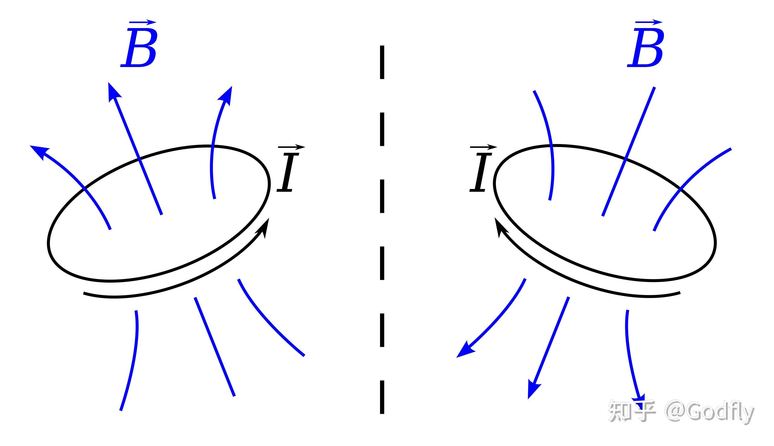
The magnetic field is a bivector. If you regard the magnetic field as a vector, this paranormal phenomenon shown in the figure arises.

In fact, the magnetic field at a point is not a vector, but a bivector; that is, \(B\in (T_pM)\wedge (T_pM)\). Its basis is \(\partial_x\wedge \partial_y,\,\partial_y\wedge \partial_z,\,\partial_z\wedge \partial_x\).

Thus, there is no paranormal event after all (welcome to Approaching Science!). Under spatial inversion, the two vectors corresponding to the magnetic field each point in the correct direction. Humans simply insist on using the right-hand screw rule to regard a bivector as a vector through Hodge duality. This is what gives rise to the strange phenomenon.

In fact, this is possible only on a three-dimensional manifold, because only there does three minus two equal one. On a four-dimensional manifold, since four minus two equals two, we cannot regard a bivector as a vector; we can only regard it as another bivector. Thus, naturally, there is no right-hand screw rule to speak of.

Of course, we still have curl on a four-dimensional manifold, except that the curl in four dimensions is a bivector rather than a vector. On an n-dimensional manifold, curl is an (n-2)-vector (see Section 3.5).

Incidentally, the electric field is also a bivector, with basis \(\partial_t\wedge \partial_x,\,\partial_t\wedge \partial_y,\,\partial_t\wedge \partial_z\), involving one time dimension. It does not appear to be a “pseudovector” because we consider only spatial inversion and not time reversal.

Pseudovectors do not exist intrinsically on a manifold. Only after equipping the manifold with a metric can we raise differential forms to pseudovector fields via the musical isomorphism. In fact, the electromagnetic field is fundamentally a differential form (a cotangent tensor field), rather than a tangent vector field. The electromagnetic field is defined as the exterior derivative \(F=\mathrm{d}A\) of the 4-potential \(A\); see Example 3.7 below.

3.7 Hodge Duality

Remark

You may have already noticed that, on an \(n\)-dimensional manifold, an \(k\)-form and an \((n-k)\)-form have the same number of basis elements! In other words, the dimension of \(\bigwedge^k(T^*M)\) equals the dimension of \(\bigwedge^{n-k}(T^*M)\). This follows from the identity \(C_n^k = C_n^{n-k}\).

If two finite-dimensional linear spaces have the same dimension, then they are isomorphic. That is, \(\bigwedge^k(T^*M)\) and \(\bigwedge^{n-k}(T^*M)\) are isomorphic, but there are infinitely many such isomorphisms. What concerns us is whether we can define a natural (canonical) isomorphism.

From the discussion in Section 2.9, we find that the structure of a smooth manifold alone cannot yield a canonical isomorphism. We need a smooth manifold equipped with an inner product (or a nondegenerate bilinear form), namely a (pseudo-)Riemannian manifold.

That is, we need to bring back our old friend—the metric. In Section 2.9, we used an inner product to induce a canonical isomorphism from the tangent bundle \(TM\) to the cotangent bundle \(T^*M\). We now use the metric to induce a canonical isomorphism from \(\bigwedge^n(T^*M)\) to \(\bigwedge^{m-n}(T^*M)\): this is Hodge duality.

Remark

All the derivations below apply not only to k-forms \(\alpha \in \bigwedge^k(T_p^*M)\), but also to k-vectors: \(v\in\bigwedge^k(T_pM)\).

Given a Riemannian manifold, we know an inner product \(V\times V\rightarrow \mathbb{R}\) on \(V\),

We now need to use it to induce an inner product \(\bigwedge^k(V)\times \bigwedge^k(V)\rightarrow \mathbb{R}\) on \(\bigwedge^k(V)\).

Let \(\alpha = \alpha_1\wedge\alpha_2\wedge \cdots\wedge \alpha_k \in \bigwedge^k(V)\), \(\beta = \beta_1\wedge\beta_2\wedge \cdots\wedge \beta_k \in \bigwedge^k(V)\). We define the inner product \(\langle\alpha\mid\beta\rangle\) on \(\bigwedge^k(V)\) as follows:

\[\langle\alpha\mid\beta\rangle= \begin{vmatrix} \langle\alpha_1\mid\beta_1\rangle & \cdots & \langle\alpha_1\mid\beta_k\rangle \\ \vdots & \ddots & \vdots \\ \langle\alpha_k\mid\beta_1\rangle & \cdots & \langle\alpha_k\mid\beta_k\rangle \end{vmatrix}\]

This definition is chosen because we want the inner product to preserve the structure of the exterior algebra.

Having defined an inner product on \(\bigwedge^k(V)\), we can derive a canonical isomorphism from \(\bigwedge^k(V)\) to \(\bigwedge^{n-k}(V)\). Next, we give the definition of this isomorphism, namely the Hodge dual:

Let \(\beta\) be an \(n\)-form on an \(m\)-dimensional manifold.

Define the Hodge dual of \(\beta\) to be an \((m-n)\)-form, denoted by \(\star \beta\), such that for every \(\alpha\in\bigwedge^{n}(T_p^*M)\)-form \(n\), the following holds:

\(\alpha \wedge (\star\beta)=\langle\alpha\mid\beta\rangle \,\omega_g\).

Here, \(\langle\cdot\mid\cdot\rangle\) is the inner product on \(\bigwedge^n(T_p^*M)\); \(\omega_g\) is the \(m\)-form formed from the orthonormal basis \(\mathrm{d}x^1\wedge \mathrm{d}x^2\wedge\cdots\wedge\mathrm{d}x^m\), also called the unit volume form. As its name suggests, its volume is 1: \(\langle \omega_g | \omega_g\rangle = 1\).

Let us restate this in plain language:

On an \(n\) -dimensional manifold, the Hodge dual \(\star \beta\) of an \(k\) -form \(\beta\) is an \((n-k)\) -form such that, for every \(k\) -form \(\alpha\) , the exterior product (volume) of \(\alpha\) and \(\star \beta\) equals the inner product of \(\alpha\) and \(\beta\).

Example 3.6

On a three-dimensional manifold, given an inner product \(\langle \mathrm{d}x^i\mid \mathrm{d}x^j\rangle=\begin{cases} 1, &i= j\\ 0, & i\neq j \end{cases}\) on \(T_p^*M\) and the induced inner product on \(\bigwedge^k(T_p^*M)\), the Hodge duals of
0-forms, 1-forms, 2-forms, and 3-forms are respectively:

\(\star f=f \,\mathrm{d}x^i \wedge\mathrm{d}x^j\wedge \mathrm{d}x^k\),
\(\star \mathrm{d}x^i =\mathrm{d}x^j\wedge \mathrm{d}x^k\),
\(\star(\mathrm{d}x^i \wedge \mathrm{d}x^j)=\mathrm{d}x^k\),
\(\star(f\,\mathrm{d}x^i \wedge\mathrm{d}x^j\wedge \mathrm{d}x^k)=f\)

Here, \((i,j,k)\) is an even permutation of \((1,2,3)\).

Please verify this yourself.

Remark

Recall the “pseudovectors” discussed in the previous section. Once Hodge duality has been defined, their relationship with bivectors becomes natural. This is precisely what we commonly call the “right-hand screw rule.”

Remark

When discussing Hodge duality, we always assume that an inner product has already been given. In other words, the inner product is prior knowledge. In this sense, Hodge duality is a natural, or canonical, isomorphism.

For physicists, Hodge duality is of course very natural. Whenever we use the right-hand screw rule, we are in fact using Hodge duality without realizing it.

Next, we give an illustration of Hodge duality in Euclidean space \(\mathbb{R}^3\):

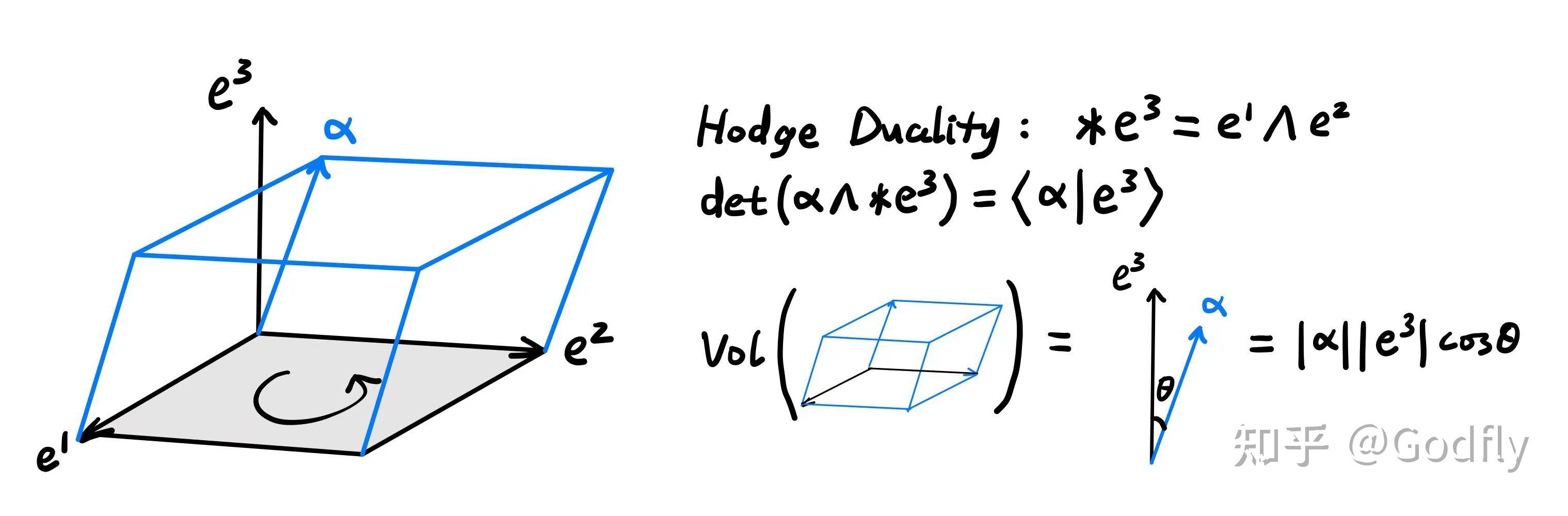
Hodge Duality

Having defined the Hodge dual, we can rewrite Maxwell’s equations in the language of exterior algebra, as shown in the following example (Example 3.7).

Example 3.7 Maxwell’s Equations (Exterior Algebra Version)

Define the electromagnetic 2-form as follows (using natural units):

\[\begin{aligned} F&=E_x\mathrm{d}t\wedge\mathrm{d}x+E_y\mathrm{d}t\wedge\mathrm{d}y+E_z\mathrm{d}t\wedge\mathrm{d}z\\ &+B_x \mathrm{d}y\wedge\mathrm{d}z + B_y \mathrm{d}z\wedge\mathrm{d}x + B_z\mathrm{d}x\wedge\mathrm{d}y \end{aligned}\]

It is in fact the exterior derivative of the 4-potential:
\(F = \mathrm{d}A\)
where \(A = -\phi/c \,\mathrm{d}t + A_x \mathrm{d}x + A_y \mathrm{d}y + A_z \mathrm{d}z\)
Readers are invited to verify this themselves.

Since the metric tensor allows us to raise or lower the indices of any tensor, raising the indices in the expression above also gives an electromagnetic tensor of type \((2,0)\), with the wedge products of \(\frac{\partial}{\partial t},\frac{\partial}{\partial x},\frac{\partial}{\partial y},\frac{\partial}{\partial z}\) as its basis. For now, however, we use the antisymmetric tensor (differential form) notation of type \((0,2)\). In any case, when a metric is provided, tensor fields of type \((2,0)\) and those of type \((0,2)\) are canonically isomorphic and may be regarded as equivalent.

Define the current differential form as follows:

\(J=-\rho c\mathrm{d}t+J_x\mathrm{d}x+J_y\mathrm{d}y+J_z\mathrm{d}z\)

As for the inner product, it is the familiar Minkowski metric:

\(\langle \mathrm{d}t\mid\mathrm{d}t\rangle=-1\)
\(\langle \mathrm{d}x\mid\mathrm{d}x\rangle=\langle \mathrm{d}y\mid\mathrm{d}y\rangle=\langle \mathrm{d}z\mid\mathrm{d}z\rangle=1\) ,
\(\langle \mathrm{d}t\mid\mathrm{d}x\rangle=\langle \mathrm{d}t\mid\mathrm{d}y\rangle=\langle \mathrm{d}t\mid\mathrm{d}z\rangle=0\) ,
\(\langle \mathrm{d}x\mid\mathrm{d}y\rangle=\langle \mathrm{d}y\mid\mathrm{d}z\rangle=\langle \mathrm{d}z\mid\mathrm{d}x\rangle=0\) ,

It induces an inner product on \(\bigwedge^2(T_p^*M)\) as follows (readers are invited to derive it themselves):

\(\langle\mathrm{d}t\wedge\mathrm{d}x\mid\mathrm{d}t\wedge\mathrm{d}x\rangle=\langle\mathrm{d}t\wedge\mathrm{d}y\mid\mathrm{d}t\wedge\mathrm{d}y\rangle=\langle\mathrm{d}t\wedge\mathrm{d}z\mid\mathrm{d}t\wedge\mathrm{d}z\rangle=-1\),
\(\langle\mathrm{d}x\wedge\mathrm{d}y\mid\mathrm{d}x\wedge\mathrm{d}y\rangle=\langle\mathrm{d}y\wedge\mathrm{d}z\mid\mathrm{d}y\wedge\mathrm{d}z\rangle=\langle\mathrm{d}z\wedge\mathrm{d}x\mid\mathrm{d}z\wedge\mathrm{d}x\rangle=1\) ,
all other terms being zero.

It also induces an inner product on \(\bigwedge^3(T_p^*M)\) as follows (readers are invited to derive it themselves):
\(\langle\mathrm{d}x\wedge\mathrm{d}y\wedge \mathrm{d}z\mid\mathrm{d}x\wedge\mathrm{d}y\wedge \mathrm{d}z\rangle=1\) ,
\(\langle\mathrm{d}t\wedge\mathrm{d}y\wedge \mathrm{d}z\mid\mathrm{d}t\wedge\mathrm{d}y\wedge \mathrm{d}z\rangle=\langle\mathrm{d}t\wedge\mathrm{d}z\wedge \mathrm{d}x\mid\mathrm{d}t\wedge\mathrm{d}z\wedge \mathrm{d}x\rangle=\langle\mathrm{d}t\wedge\mathrm{d}x\wedge \mathrm{d}y\mid\mathrm{d}t\wedge\mathrm{d}x\wedge \mathrm{d}y\rangle=-1\)
all other terms being zero.

Under the inner product above (the Minkowski metric), Maxwell’s equations can be written as follows:

\[\left\{\quad \begin{aligned} \mathrm{d}F&=0\\ \star\,\mathrm{d}\star F &= J \end{aligned} \right.\]

Interested readers may derive the equation above themselves. The calculation is not complicated. Here, \(\mathrm{d} F = 0\) is immediate, because \(F = \mathrm{d}A\) whereas \(\mathrm{d}\mathrm{d} = 0\) .

Summary

In this chapter, we studied differentiation on manifolds using exterior algebra. Specifically:

First, we introduced alternating multilinear maps and defined the wedge product from them. Taking the direct sum of exterior products of degree 0, 1, …, n gives the exterior algebra.

Second, we introduced forms, which live in the exterior algebra of the cotangent space. Differential forms are “fields of forms”: a form is assigned to every point on a manifold. We also introduced the exterior derivative operator, which generalizes differentiation to exterior algebra.

Finally, we applied the theory above to familiar concepts such as the gradient, curl, divergence, pseudovectors, and pseudoscalars, and then introduced the notion of the Hodge dual. The Hodge dual naturally connects the inner product and the exterior product. In particular, on a three-dimensional manifold, it can also induce the cross product. Every time we use the cross product and the right-hand screw rule, we are using the Hodge dual.

Chapter 4 Derivatives on Manifolds

In Chapter 3, we studied the exterior differential (also called the exterior derivative, because its English name is exterior derivative). In this chapter, we introduce two other kinds of derivatives: the covariant derivative and the Lie derivative.

Both the covariant derivative and the Lie derivative differentiate one tensor field with respect to another tangent vector field; that is, both describe the change of a tensor along the direction of another tangent vector. The difference is that the Lie derivative depends on the behavior of the other tangent vector field in a neighborhood, whereas the covariant derivative does not. However, a covariant derivative requires a metric in order to be uniquely determined.

4.1 Covariant Derivative and Connection

Comment

Although we defined tangent spaces in Section 2.1, thereby giving vectors on a manifold a place to live, we still cannot directly compare tangent vectors at two points, because the tangent space at point p and that at point q are two different spaces.

If we cannot do this, the consequences are serious. Consider acceleration in classical mechanics: to define it, we need to compare velocities at times \(t\) and \(t+\epsilon\), but these two velocity vectors lie in different tangent spaces. If we cannot compare these velocity vectors, we cannot even define acceleration!

To compare a vector at point p with a vector at point q, we must find a way to parallel transport the vector at p to q. To make this operation possible, we need a connection. A connection can be characterized by a covariant derivative.

The reason we do not notice this issue in Euclidean space is that Euclidean space has a very natural translation operation—so natural that we fail to realize we use it every day.

For a vector \(u\) at a point \(p\) on a manifold \(M\), its covariant derivative along another vector \(v\) is denoted by \(\nabla_v u\). It is also a vector at the point \(p\). It represents the change in the vector \(u\) along the vector \(v\).

In fact, the covariant derivative acts on two vector fields: \(\nabla_W A\), and yields another vector field. In the context above, \(u\) belongs to the vector field \(A\), and \(v\) belongs to the vector field \(W\).

The covariant derivative \(\nabla_W\) can act not only on vector fields \(A\), but can also be extended to general tensor fields (including scalar fields, since scalar fields are also a special type of tensor field). We now give the definition of the covariant derivative:

A covariant derivative is a map \(\mathcal{T}^m_n(M)\rightarrow \mathcal{T}^m_n(M)\) satisfying the following properties:

1. Linearity: \( \nabla_W(\lambda A+\mu B) = \lambda \nabla_W A + \mu \nabla_W B \)
2. \(\mathcal{F}\)-linearity in \(W\): \( \nabla_{V+fW} = \nabla_V + f\nabla_W \quad f\in\mathcal{F}(M) \)
3. Leibniz rule: \( \nabla_W(A\otimes B) = (\nabla_W A)\otimes B + A \otimes (\nabla_W B) \)
4. It commutes with contraction: \( \nabla_W \circ C = C \circ \nabla_W \)
5. For a scalar field \(f\), the action of \(\nabla_W\) on \(f\) is equivalent to that of \(W\) on \(f\) (see Section 2.2): \( \nabla_W f = Wf \)

Now, in the expression \(\nabla_W A\), let \(W=e_k\), where \(e_k\) is the vector field formed by one basis vector of a coordinate system; then let \(A=e_j\), where \(e_j\) is the vector field formed by another basis vector of the coordinate system. Then the action of \(\nabla_{W}\) on \(A\) can be written as \(\nabla_{e_k}e_j\), which we abbreviate as \(\nabla_{k} e_j\). Since \(\nabla_{k} e_j\) is also a vector field, we can write it as a linear combination of vectors: \(\nabla_{k} e_j = \Gamma^i_{jk}e_i.\)

\(\Gamma^i_{jk}\) is the famous Christoffel symbol. It is also sometimes called a linear connection.

It can be proved that \(\Gamma^i_{jk}\) uniquely determines a covariant derivative. This follows from the five properties in the definition of the covariant derivative; the proof is omitted.

Comment

Pause for a moment and consider the meanings of the three subscripts of \(\Gamma^i_{jk}\): \(k\) represents motion along the \(k\)th direction, \(j\) indicates that we are considering the change of the \(j\)th basis vector, and \(i\) represents the component of that change along the \(i\)th basis vector.

Note

It can be proved that \(\Gamma^i_{jk}\) is not a tensor. Mathematically, the component representation of a tensor is merely its representation; under a coordinate transformation, the tensor itself remains unchanged, and only the coordinates change. However, \(\Gamma^i_{jk}\) itself changes with the coordinate system—it does not obey the tensor transformation law.

Some authors nevertheless hold that, in the context of a fixed coordinate system, the Christoffel symbols may be called a tensor, or a “coordinate-dependent tensor.” Such terminology is not very rigorous, so we will not adopt it here.

We now discuss how to compute covariant derivatives.

For a tangent vector field \(A^j\partial_j\), since we already know \(\nabla_k\partial_j = \Gamma^i_{jk} \partial_i\), its covariant derivative is easy to compute:

Example 4.1

Compute the covariant derivative \(\nabla_W A\) of the tangent vector field \(A = A^j\partial_j\).

Solution:

\( \begin{aligned} \nabla_W A &= \nabla_{W^k\partial_k}(A^j\partial_j) \\ &\stackrel{2}{=} W^k \nabla_k (A^j\partial_j) \\ &\stackrel{3,4}{=} W^k (\nabla_k A^j \partial_j + A^j \nabla_k \partial_j ) \\ &\stackrel{5}{=} W^k (\partial_k A^j \partial_j + A^j \nabla_k \partial_j ) \\ &:= W^k (\partial_k A^j \partial_j + A^j \Gamma^l_{jk}\partial_l) \\ &= W^k (\partial_k A^l + A^j \Gamma^l_{jk}) \partial_l \end{aligned} \)

The numbers above the equality signs indicate which property was used.

Thus, the components of \(\nabla_W A\) in \(\partial_l\) are:

\( (\nabla_W A)^l = W^k (\partial_k A^l + \Gamma_{jk}^l A^j) \)

The expression above shows that the covariant derivative \(\nabla_W A\) differs from the derivative of the components \(W^k\partial_k A\) by a Christoffel-symbol term.

Having computed the covariant derivative of a tangent vector field, we now compute the covariant derivative \(\nabla_W \alpha\) of a cotangent vector field \(\alpha = \alpha_j\mathrm{d}x^j\).

We first compute the expression for the action of \(\nabla_k\) on a basis covector \(\mathrm{d}x^j\), namely the expression for \(\nabla_k \mathrm{d}x^j\).

Example 4.2

Compute \(\nabla_k \mathrm{d}x^j\).

Solution:

Since the covariant derivative commutes with tensor contraction and satisfies the Leibniz rule,

\( \nabla_k(\alpha(A)) = (\nabla_k\alpha)A + \alpha(\nabla_k A) \)

Choose \(\alpha = \mathrm{d}x^i\) and \(A=\partial_j\). Then

\( \nabla_k(\mathrm{d}x^i(\partial_j)) = (\nabla_k \mathrm{d}x^i)\partial_j + \mathrm{d}x^i(\nabla_k \partial_j) \)

Note that, in the expression above, we have contracted a tensor of type \((1,1)\). Therefore, \(\mathrm{d}x^i(\partial_j)\) on the left-hand side is a constant scalar field (identically either 1 or 0), and hence \( \nabla_k(\mathrm{d}x^i(\partial_j))\) on the left-hand side is the zero scalar field.

Rearranging terms (and taking the contraction into account) gives

\( \nabla_k \mathrm{d}x^i = -\Gamma^i_{jk}\mathrm{d}x^j \)

Furthermore,

\( \nabla_W \mathrm{d}x^i = -(\Gamma^i_{jk}W^k)\mathrm{d}x^j \)

For a general cotangent vector field \(\alpha = \alpha_j\mathrm{d}x^j\), the derivation of its covariant derivative is left as an exercise. Hint: follow the method of Example 4.1.

We now have the covariant derivatives of tangent and cotangent vector fields. How, then, should we compute the covariant derivative \((\nabla_W A)^{i...j}_{k...l}\) of a general tensor of type \((p,q)\)? We give the formula directly here. Interested readers may derive it themselves using the method of Example 4.1 and the result of Example 4.2:

Example 4.3

Compute the covariant derivative \((\nabla_W A)^{i...j}_{k...l}\) of the tensor \(A\).

Solution (derivation omitted):

\( \begin{aligned} (\nabla_W A)^{i...j}_{k...l} & = W^{m} \partial_{m} A^{i...j}_{k...l} \\ & - \Gamma^{n}_{km} W^{m} A^{i...j}_{n...l} - \cdots - \Gamma^{n}_{lm} W^m A^{i...j}_{k...n} \\ & + \Gamma^{i}_{nm} W^{m} A^{n...j}_{k...l} + \cdots + \Gamma^{j}_{nm} W^m A^{i...n}_{k...l} \end{aligned} \)

4.2 Riemann–Levi-Civita Connection

Comment

So far, for a given manifold, there are many covariant derivatives satisfying the five properties above. How can we find a unique covariant derivative?

You may immediately think of a metric. Indeed, without a metric, the choice of covariant derivative is rather arbitrary. We have no reason to choose a particular covariant derivative—or, equivalently, no reason to choose a particular connection \(\Gamma^i_{jk}\).

In fact, however, to induce a unique covariant derivative, we need not only a metric but also torsion-freeness. Therefore, we first introduce torsion-freeness.

The torsion-free condition for a covariant derivative \(\nabla\) is defined as follows:

\[ \nabla_V W - \nabla_W V = [V, W] \]

If \(\nabla\) satisfies the equation above, then we call \(\nabla\) torsion-free.

Remark

\([V, W]\) is defined as \([V, W]: [V, W]f = V(W(f))-W(V(f))\)

It is worth noting that, in general, \(VW : VW(f)=V(W(f))\) is not a vector field. However, \(VW-WV\) is indeed a vector field; see Section 4.8.

Remark

Although \(\Gamma^i_{jk}: \nabla_k e_j = \Gamma^i_{jk} e_i \) is not a tensor, \(T(V,W) := \nabla_V W - \nabla_W V - [V, W]\) is indeed a tensor, called the torsion tensor; the proof is omitted.

For every covariant derivative, we can define a torsion tensor. When the torsion tensor vanishes, we say that the covariant derivative is torsion-free.

It can be shown that the components of \(T(V,W)\) in \(e^i\) are \( T^{i}_{jk}=\Gamma^{i}_{kj}-\Gamma^{i}_{jk} \). Setting \(T(V,W)\) to zero, we obtain
\( \Gamma^i_{jk} = \Gamma^i_{kj} \)

The torsion-free condition for a covariant derivative is expressed by \( \Gamma^i_{jk} = \Gamma^i_{kj} \).

Remark

It is easy to see that \(T(V,W)\) is an antisymmetric tensor. Setting it to zero gives \(n\cdot n(n-1)/2\) constraints (for the three indices \(i,j,k\)), where \(n\) is the dimension of the manifold.

Remark

Torsion-freeness can also be defined as follows: \(\nabla_a\nabla_b f=\nabla_b\nabla_a f\), where \(f\in \mathcal{F}(M)\) is a scalar field. This definition is equivalent to the one above.

By imposing torsion-freeness, we restrict the number of possible covariant derivatives, but not yet to a unique one. Next, we consider the metric in order to narrow the possible covariant derivatives down to one.

Remark

To determine a covariant derivative uniquely, we need \(n^3\) constraints. Above, we have already obtained \(n\cdot n(n-1)/2\) constraints. Next, we need another \(n\cdot n(n+1)/2\) constraints, which follow from metric compatibility.

We now require that the covariant derivative preserve the metric, or equivalently, satisfy metric compatibility. This is because we want the length of a vector to remain unchanged as it is transported along a curve. In other words, we require the covariant derivative of the metric tensor to vanish:

\[ \nabla_k g_{ij}=0 \]

Example 4.4

Derive the Christoffel symbols for a torsion-free, metric-compatible covariant derivative. In other words, express \(\Gamma^i_{ij}\) in terms of \(g_{ij}\).

Solution:

According to Example 4.3, we can write the covariant derivative of the metric tensor as:

\( \nabla_k g_{ij} = \partial_k g_{ij} - \Gamma^l_{ik}g_{lj} - \Gamma^l_{jk}g_{il} \)

We now define the Christoffel symbols of the first kind as \(\Gamma_{ijk} = g_{il}\Gamma^l_{jk}\). The Christoffel symbols \(\Gamma^{i}_{jk}\) introduced earlier are the Christoffel symbols of the second kind.

After defining the Christoffel symbols of the first kind \(\Gamma_{ijk}\), the above expression can be written as:

\( \nabla_k g_{ij} = \partial_k g_{ij} - \Gamma_{jik} - \Gamma_{ijk} \)

Let \(\nabla_k g_{ij} = 0\), then we have

\( \partial_k g_{ij} = \Gamma_{ijk} + \Gamma_{jik} \)

Moreover, torsion-freeness gives

\( \Gamma_{ijk} - \Gamma_{ikj} = 0 \)

Combining the two equations above, we can solve for the Christoffel symbols of the first kind:

\( \Gamma_{ijk} = \frac{1}{2}(g_{ij,k} + g_{ik,j} - g_{jk,i}) \)

where \(g_{ij,k}:=\partial_k g_{ij}\). From this, we can obtain the Christoffel symbols of the second kind:

\( \Gamma^i_{jk} = \frac{g^{il}}{2}(g_{lj,k}+g_{lk,j}-g_{jk,l}) \)

Thus, once torsion-freeness and metric compatibility are specified, the covariant derivative is uniquely determined. The connection \(\Gamma^i_{ij}\) corresponding to this covariant derivative is called the Riemann connection or the Levi-Civita connection.

Since three people’s names are involved, we may as well call it the Riemann-Levi-Civita connection, or the RLC connection, incorporating the initials of all three names. Note that RLC does not stand for resistance, inductance, and capacitance!

The RLC connection is given by \( \Gamma^i_{jk} = \frac{g^{il}}{2}(g_{lj,k}+g_{lk,j}-g_{jk,l})\).

4.3 Parallel Transport

Remark

Once a connection (covariant derivative) is given, we can define parallel transport. This is also the original purpose of defining a connection: to compare vectors at different points.

Parallel transport is defined as follows:

Given a curve \(\gamma: [0,T] \rightarrow M\) on \(M\), and a vector \(V_0 \in T_{\gamma(0)}M\) at the point \(\gamma(0)\), define the parallel transport \(V(t)\) of \(V_0\) along the curve \(\gamma(t)\) as the solution to the following equation:

\[ \nabla_{\gamma^\prime(t)}V(t) = 0 \]

where \(t\in[0,T]\) and \(V(0)=V_0\).

Remark

A covariant derivative represents the change of a vector, whereas parallel transport requires the vector not to change as it moves. Therefore, we can define parallel transport by requiring that the covariant derivative along the curve vanish.

Next, we derive the coordinate expression for parallel transport. To do so, we need to expand \(\nabla_{\gamma^\prime(t)}V(t)\) (see Example 4.1):

\[ \begin{aligned} \nabla_{\gamma^\prime(t)}V(t) &= \nabla_{\frac{\mathrm{d}\gamma^k}{\mathrm{d}t}\partial_k}(V^j(t)\partial_j) \\ & = \frac{\mathrm{d}\gamma^k}{\mathrm{d}t} (\partial_k V^j \partial_j + V^j \Gamma^i_{jk} \partial_i) \\ & = \frac{\mathrm{d}V^j}{\mathrm{d}t} \partial_j + \frac{\mathrm{d}\gamma^k}{\mathrm{d}t} V^j \Gamma^i_{jk} \partial_i \\ & = \left(\frac{\mathrm{d}V^i}{\mathrm{d}t} + \frac{\mathrm{d}\gamma^k}{\mathrm{d}t} V^j \Gamma^i_{jk} \right)\partial_i \end{aligned} \]

Let \(\nabla_{\gamma^\prime(t)}V(t) = 0\), then:

\[\begin{aligned} \frac{\mathrm{d}V^i}{\mathrm{d}t} + \Gamma^i_{jk} \frac{\mathrm{d}\gamma^k}{\mathrm{d}t} V^j = 0 \end{aligned}\]

This is the parallel transport equation. It is a system of first-order ordinary differential equations in \(V^i\). Solving it yields the coordinate components of the vector \(V\) after parallel transport along the curve \(\gamma\).

4.4 Geodesics

Remark

Recall Newton’s first law. It states that a particle subject to no external forces maintains a constant velocity. In other words, its acceleration is zero.

When the particle is in the familiar Euclidean space, because Euclidean space has a very natural connection, we can easily parallel transport the velocity vector. Such transport leads to the conclusion that the particle moves along a straight line (or remains at rest).

However, on a general manifold, the situation is different: parallel transport of a velocity vector is no longer as natural and trivial as in Euclidean space. Consequently, the trajectory of the particle is no longer a simple straight line in Euclidean space. In fact, we have not even defined what a “straight line” on a manifold is.

Fortunately, we can use the idea of Newton’s first law to define “straight lines” on a manifold, calling them geodesics. Specifically, we define a geodesic as the trajectory of a particle with zero acceleration.

Before that, however, we first need to define acceleration.

Given a curve \(\gamma: [0, T] \rightarrow M\) on \(M\), its acceleration at the point \(\gamma(t)\) is defined as:

\[ a(t) = \nabla_{\gamma^\prime(t)}\gamma^\prime(t) = \nabla_{v(t)}v(t) \]

where \(v(t):=\gamma^\prime(t)\) is the velocity of the curve at the point \(\gamma(t)\).

If the acceleration of a curve is zero everywhere, then the curve is called a geodesic, that is:

\[ \nabla_{\gamma^\prime(t)}\gamma^\prime(t) = 0 \]

Next, let us examine the coordinate representation of acceleration:

\[ \begin{aligned} \nabla_{v(t)}v(t) & = v^k \nabla_k (v^j\partial_j) \\ & = v^k (\nabla_k v^j \partial_j + v^j \nabla_k \partial_j ) \\ & = v^k (\partial_k v^j \partial_j + v^j \Gamma^i_{jk} \partial_i) \\ & = v^k (\partial_k v^i + v^j \Gamma^i_{jk}) \partial_i \\ & = \left(\frac{\mathrm{d} v^i}{\mathrm{d}t} + \Gamma^i_{jk} v^j v^k \right) \partial_i \end{aligned} \]

Setting the acceleration equal to zero, we obtain:

\[\begin{aligned} \frac{\mathrm{d} v^i}{\mathrm{d}t} = -\Gamma^i_{jk}v^jv^k \end{aligned}\]

This is the geodesic equation. Writing \(v^i\) as \(\frac{\mathrm{d} \gamma^i}{\mathrm{d}t}\), we have

\[\begin{aligned} \frac{\mathrm{d}^2 \gamma^i}{\mathrm{d}t^2} = -\Gamma^i_{jk}\frac{\mathrm{d} \gamma^j}{\mathrm{d}t}\frac{\mathrm{d} \gamma^k}{\mathrm{d}t} \end{aligned}\]

Clearly, this is a system of second-order ordinary differential equations in \(\gamma(t)\). Solving it gives the equations of geodesics on the manifold.

4.5 Curvature

Remark

In general, transporting a vector at the point \(p\) to the point \(q\) along different paths yields different results. This phenomenon is called holonomy and leads to the concept of curvature. See the figure below:

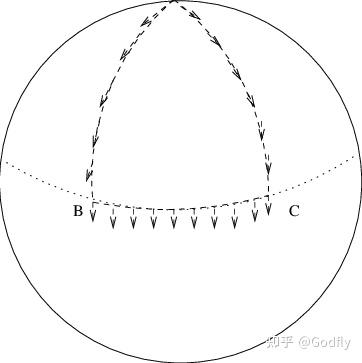
A vector at the North Pole is first transported along a meridian to the equator, then along the equator, and finally back to the North Pole along a meridian; it does not coincide with its initial state.

Now, let us consider a loop along the coordinate axes, as shown below:

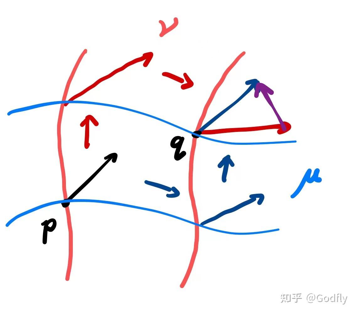
A vector at point p is parallel transported to point q along two different paths, yielding different results.

As shown in the figure, a vector at point \(p\) is parallel transported to point \(q\) along two different paths. These two paths are:

1. First vary \(x_\nu\), then vary \(x_\mu\);

2. First vary \(x_\mu\), then vary \(x_\nu\).

As this loop is continuously shrunk, the difference between the results of parallel transporting a basis tangent vector \(e_\beta\) along these two paths can be written as:

\[ \begin{aligned} & \phantom{=} \nabla_\mu\nabla_\nu e_\beta - \nabla_\nu\nabla_\mu e_\beta \\ & = \nabla_\mu(\Gamma^{\alpha}_{\beta\nu}e_\alpha) - \nabla_\nu(\Gamma^{\alpha}_{\beta\mu}e_\alpha) \\ & = (\partial_\mu\Gamma^{\alpha}_{\beta\nu}) + \Gamma^{\alpha}_{\beta\nu}(\nabla_\mu e_\alpha) - (\nabla_\nu\Gamma^{\alpha}_{\beta\mu})e_\alpha - \Gamma^{\alpha}_{\beta\mu}(\nabla_\nu e_\alpha)\\ & = (\Gamma^{\alpha}_{\beta\nu,\mu} + \Gamma^\lambda_{\beta\nu}\Gamma^{\alpha}_{\lambda\mu} - \Gamma^{\alpha}_{\beta\mu,\nu} - \Gamma^\lambda_{\beta\mu}\Gamma^{\alpha}_{\lambda\nu}) e_\alpha \end{aligned} \]

\(\Gamma^{\alpha}_{\beta\nu,\mu}\) denotes \(\partial_\mu \Gamma^{\alpha}_{\beta\nu}\). This is a convention: a comma \(A_{,\alpha}\) denotes the partial derivative with respect to a component, \(\partial_\alpha A\).
Sometimes, we also use a semicolon \(A_{;\alpha}\) to denote a covariant derivative, \(\nabla_\alpha A\).

Let \(R^{\alpha}_{\beta\mu\nu} = \Gamma^{\alpha}_{\beta\nu,\mu} - \Gamma^{\alpha}_{\beta\mu,\nu} + \Gamma^\lambda_{\beta\nu}\Gamma^{\alpha}_{\lambda\mu} - \Gamma^\lambda_{\beta\mu}\Gamma^{\alpha}_{\lambda\nu}\). It can be shown that \(R^{\alpha}_{\beta\mu\nu}\) is a tensor. We call it the Riemann Curvature Tensor.

In other words, the Riemann tensor is defined as:

\[ \begin{aligned} R^{\alpha}_{\beta\mu\nu} & := (\nabla_\mu\nabla_\nu e_\beta - \nabla_\nu\nabla_\mu e_\beta)^\alpha \\ & = \Gamma^{\alpha}_{\beta\nu,\mu} - \Gamma^{\alpha}_{\beta\mu,\nu} + \Gamma^\lambda_{\beta\nu}\Gamma^{\alpha}_{\lambda\mu} - \Gamma^\lambda_{\beta\mu}\Gamma^{\alpha}_{\lambda\nu} \end{aligned} \]

Comment

Let us pause to consider the geometric meaning of the Riemann curvature tensor \(R^{\alpha}_{\beta\mu\nu}\). It represents the \(\alpha\)th component of the difference between the results obtained by transporting the \(\beta\)th basis vector along two different paths (first along \(x_\mu\) and first along \(x_\nu\)).

From the definition of the Riemann curvature tensor, we immediately obtain one of its properties: \(R^\alpha_{\beta\mu\nu}\) = \(R^\alpha_{\beta\nu\mu}\). Using this property, the number of independent components can be reduced from \(n^4\) to \(n^3(n+1)/2\). In fact, however, the Riemann curvature tensor satisfies further properties, which reduce the number of independent components to \(n^2(n^2-1)/12\). We will not introduce these properties here; interested readers may consult relevant textbooks.

Next, we can define the Ricci Tensor:

\[ R_{\beta\nu} := R^\lambda_{\beta \lambda \nu} \]

The Ricci tensor is obtained by contracting the Riemann curvature tensor. As for why \(\alpha\) is contracted with \(\mu\) rather than with \(\nu\), the reason is that the two differ only by a minus sign; contraction with either \(\mu\) or \(\nu\) is possible.

If \(\alpha\) is contracted with \(\beta\), the result is zero; the proof is omitted.

The Ricci tensor is symmetric: \(R_{\mu\nu}=R_{\mu\nu}\); the proof is omitted.

Finally, using the metric, we can obtain the Ricci scalar (Ricci curvature), also called the scalar curvature:

\[ R = g^{\mu\nu}R_{\mu\nu} \]

4.6 Introduction to General Relativity

The core of general relativity—the Einstein field equations—gives the relationship between spacetime curvature and the motion of matter. The former describes how spacetime curves, while the latter describes the evolution of energy and momentum in spacetime.

Define the Einstein tensor \(G_{\mu\nu} := R_{\mu\nu}-\frac{1}{2}Rg_{\mu\nu}\). Then the Einstein field equations can be written as:

\[ G_{\mu\nu} = \frac{8\pi G}{c^4} T_{\mu\nu} \]

Here, \(T_{\mu\nu}\) is called the energy-momentum tensor.

Let us explain the energy-momentum tensor, which has 16 components:

\[ T = \begin{pmatrix} T_{tt} & T_{tx} & T_{ty} & T_{tz} \\ T_{xt} & T_{xx} & T_{xy} & T_{xz} \\ T_{yt} & T_{yx} & T_{yy} & T_{yz} \\ T_{zt} & T_{zx} & T_{zy} & T_{zz} \end{pmatrix} \]

Here, \(T_{tt}\) represents the energy density, \((T_{tx}, T_{ty}, T_{tz})\) represents the momentum density, and

\[ \begin{pmatrix} T_{xx} & T_{xy} & T_{xz} \\ T_{yx} & T_{yy} & T_{yz} \\ T_{zx} & T_{zy} & T_{zz} \end{pmatrix} \]

represents the stress tensor. In particular, the diagonal elements \(T_{xx},T_{yy},T_{zz}\) represent the pressures in the three respective directions.

Comment

In the Einstein field equations \(G_{ab} = 8\pi T_{ab}\) (in natural units), the left-hand side describes how spacetime curves, while the right-hand side describes how matter evolves.

Just as Maxwell’s equations are the fundamental postulates of electrodynamics, the Einstein field equations are the fundamental postulates of general relativity. They cannot be derived from other equations.

If we regard electrodynamics as Maxwell’s equations + solving them + applications, then in some sense we can likewise say that general relativity is Einstein’s field equations + solving them + applications.

Example 4.5 The Schwarzschild Metric and the Schwarzschild Black Hole

The Schwarzschild metric describes the spacetime surrounding a spherical body with no charge, no angular momentum, and mass \(M\):

\( \left\{\begin{aligned} g_{tt} &= - (c^2 - \frac{2GM}{r}) \\ g_{rr} &= \frac{1}{1-\frac{2GM}{rc^2}} \\ g_{\theta\theta} &= r^2 \\ g_{\varphi\varphi} &= r^2 \sin^2 \theta \\ g_{\text{otherwise}} &= 0 \end{aligned}\right. \)

It was the first nontrivial exact solution to the Einstein field equations. Note that \(r=\frac{2GM}{c^2}\) is a singularity of the metric. Of course, since the Schwarzschild metric applies only to the spacetime outside the spherical body, this is not a problem when the radius of the body is \(R\gt \frac{2GM}{c^2}\).

However, if the radius of the body is \(R\lt \frac{2GM}{c^2}\), an object outside the body may pass through \(r=\frac{2GM}{c^2}\).

Moreover, when \(r\lt \frac{2GM}{c^2}\), \(g_{rr}\) changes from positive to negative, and \(g_{tt}\) changes from negative to positive. In other words, \(r\) becomes a timelike coordinate, meaning that, in a sense, the radial spatial dimension becomes a time dimension: falling toward the center becomes an unavoidable future.

Therefore, when \(R\lt \frac{2GM}{c^2}\), the spherical body collapses into a very small point (in the model of general relativity). This is the commonly known Schwarzschild black hole. The spherical surface at \(r=\frac{2GM}{c^2}\) is called the event horizon.

The derivation of the Schwarzschild solution is too lengthy to present here.

4.7 Pull-back and Push-Forward

Comment

Pull-back and push-forward are very useful concepts. They are used in many of the concepts introduced later. Therefore, it is well worthwhile to devote a separate section to them.

Let us now consider a smooth map \(\phi: M\rightarrow N\) from a manifold \(M\) to a manifold \(N\). If there is a scalar field \(f\) on \(N\), then, with the aid of \(\phi\), we can induce a scalar field on \(M\):

\[ \phi^* f := f \circ \phi \]

Here, \(\phi^*\) is called the pull-back. As its name suggests, it “pulls back” the domain of \(f\) from \(N\) to \(M\).

Comment

One point should be noted: we have not assumed that \(\phi\) is a bijection. In fact, \(\phi\) need be neither injective nor surjective. So far, the only requirement we impose on \(\phi\) is that it be smooth.

Now let us consider whether, given a scalar field on \(M\), we can use \(\phi\) to “push it forward” to \(N\). The answer is no, because \(\phi\) need not be injective; that is, multiple points on \(M\) may be mapped to the same point on \(N\). Therefore, without injectivity, we cannot define the “push-forward” of a scalar field.

Of course, we could simply assume that \(\phi\) is a diffeomorphism, and then define the push-forward straightforwardly. But before doing so, let us first see how to define the push-forward and pull-back of tangent vectors, cotangent vectors, and tensors. Please be patient, because we want to know what happens when \(\phi\) is not a bijection.

We now consider the push-forward of tangent vectors. Using the pull-back of scalar fields, we can define the push-forward of a tangent vector at a point:

\[ \begin{aligned} \phi_{*}: T_{p} M &\rightarrow T_{\phi(p)} N \\ (\phi_{*} v)|_{\phi(p)} f &:= v|_p(\phi^{*} f) \quad \forall f \end{aligned} \]

Optional Reading 4.1

The push-forward can also be defined using the alternative definition of tangent vectors—as equivalence classes of curves. Consider a curve \(\gamma\) on \(M\) passing through the point \(p\). This curve is mapped by \(\phi\) to a curve \(\phi \circ \gamma\) on \(N\) passing through the point \(\phi(p)\). We want the vector on \(M\) tangent to the curve \(\gamma\) at \(p\) to be pushed forward by \(\phi\) to a vector on \(N\) that is likewise tangent to \(\phi \circ \gamma\) at \(\phi(p)\). Recall that a tangent vector at \(p\) can also be defined as an equivalence class of curves \([\gamma]\), namely, all curves with the same derivative at \(p\). We may therefore define the push-forward map as follows:

\( \phi_*[\gamma] := [\phi \circ \gamma] \)

Put simply, the tangent vector of a curve is pushed forward to the tangent vector of its image curve.

Comment

Since \(\phi\) need be neither injective nor surjective, we still cannot define the push-forward of a vector field; we can define only the push-forward of a vector at a point. This is because:

a. If \(\phi\) is not surjective, vectors on \(M\) can be pushed forward only to the image of \(N\) in \(\phi\). Thus, the vector field on \(N\) is defined only on the subset \(\mathrm{Im}(\phi)\).
b. If \(\phi\) is not injective, vectors at two distinct points on \(M\) may be pushed forward to the same point on \(N\), and these two vectors need not be equal.

Comment

We have just defined the push-forward of tangent vectors using the pull-back of scalars. Next, we use the push-forward of tangent vectors to define the pull-back of cotangent vectors.

We now consider the pull-back of cotangent vectors. Using the push-forward of tangent vectors, we can define the pull-back of a cotangent vector field:

\[ \begin{aligned} \phi^*: \mathcal{T}^0_1(N) &\rightarrow \mathcal{T}^0_1(M) \\ \phi^*\omega(v|_p) &:= \omega((\phi_* v)|_{\phi(p)}) \end{aligned} \]

Remark

Notice that in this definition, we can define the pullback not only of a cotangent vector at a single point, but also of all cotangent vectors on the manifold \(N\). In other words, even when \(\phi\) is not a diffeomorphism, we can still define the pullback of a cotangent vector field.

This may seem remarkable, but on reflection it is entirely natural: if we can pull back a scalar field, then we should also be able to pull back the differential of that scalar field, and the differential is a cotangent vector field.

By the same reasoning, we can define the pullback of a tensor field of type \((0,n)\):

\[ \begin{aligned} \phi^*: \mathcal{T}^0_l(N) &\rightarrow \mathcal{T}^0_l(M) \\ \phi^*T(v^1|_p, \cdots, v^n|_p) &:= T((\phi_* v^1)|_{\phi(p)}, \cdots, (\phi_* v^n)|_{\phi(p)}) \end{aligned} \]

Remark

So far, we have defined the pullback of scalar fields, the pushforward of tangent vectors (note: not tangent vector fields), the pullback of cotangent vector fields, and the pullback of tensor fields of type \((0,n)\). Next, we define the pushforward of tensors of type \((l,0)\) (note: not tensor fields).

We now define the pushforward of a tensor of type \((m,0)\) at a point:

\[ \begin{aligned} \phi_*: T^m_0|_pM &\rightarrow T^m_0|_p N \\ (\phi_* T)|_{\phi(p)}(\omega_1, \cdots, \omega_m) &:= T|_{p}(\phi^* \omega_1, \cdots, \phi^* \omega_m) \end{aligned} \]

Remark

The reason we cannot define the pushforward of a “field” for tangent vectors and tensors of type \((m,0)\) is again the reason mentioned earlier: \(\phi\) need not be bijective.

If \(\phi\) is not bijective (i.e., not a diffeomorphism), this is the best we can do. We therefore next impose the additional condition that \(\phi\) is a diffeomorphism. In that case, we can define both pullbacks and pushforwards of tensor fields of any type.

We now upgrade \(\phi\) from a smooth map from \(M\) to \(N\) to a diffeomorphism from \(M\) to \(N\). We can then define the pushforward of tangent vector fields and tensor fields of type \((m,0)\):

\[ \begin{aligned} \phi_*: \mathcal{T}^m_0(M) &\rightarrow \mathcal{T}^m_0(N) \\ (\phi_* T)(\omega_1, \cdots, \omega_m) &:= T(\phi^* \omega_1, \cdots, \phi^* \omega_m) \end{aligned} \]

Moreover, we can define the pullback of tensor fields of type \((m,0)\), because we can interchange the roles of \(M\) and \(N\): the pullback via \(\phi\) can be regarded as the pushforward via \(\phi^{-1}\), namely \(\phi^*=(\phi^{-1})_*\):

\[ \begin{aligned} \phi_*: \mathcal{T}^m_0(N) &\rightarrow \mathcal{T}^m_0(M) \\ (\phi^* T)(\omega_1, \cdots, \omega_m) &= ((\phi^{-1})_* T)(\omega_1, \cdots, \omega_m) \\ &:= T((\phi^{-1})^* \omega_1, \cdots, (\phi^{-1})^* \omega_m) \end{aligned} \]

On this basis, we can define the pullback of tensor fields of type \((m,n)\):

\[ \begin{aligned} \phi^*: \mathcal{T}^m_n(N) &\rightarrow \mathcal{T}^m_n(M) \\ (\phi^* T)(\omega_1, \cdots, \omega_m, v^1, \cdots, v^n) &= T(\phi_* \omega_1, \cdots, \phi_* \omega_m, (\phi^{-1})^* v^1, \cdots, (\phi^{-1})^* v^n) \end{aligned} \]

The pushforward of a tensor field of type \((m,n)\) is obtained simply by substituting \(\phi^*=(\phi^{-1})_{*}\) into the above expression:

\[ \begin{aligned} \phi_*: \mathcal{T}^m_n(M) &\rightarrow \mathcal{T}^m_n(N) \\ (\phi_* T)(\omega_1, \cdots, \omega_m, v^1, \cdots, v^n) &= T((\phi^{-1})_* \omega_1, \cdots, (\phi^{-1})_* \omega_m, \phi^* v^1, \cdots, \phi^* v^n) \end{aligned} \]

Finally, readers are invited to derive the explicit computational formulas for pullback and pushforward maps themselves. As in Example 2.6, the results involve the Jacobian matrix.

4.8 Lie Derivative

Remark

Our introduction to covariant derivatives now comes to an end. Next, we introduce another kind of derivative, called the Lie derivative. Before that, however, we need to introduce several more concepts.

We begin by defining an integral curve. Given a tangent vector field, an integral curve is a curve whose derivative at every point equals the tangent vector at that point.

The electric field lines we commonly speak of are integral curves of the electric field.

Countless integral curves resemble a river. If we “go with the flow,” we drift from one point on the manifold to another:

\[ \Phi_t: M\rightarrow M \quad \gamma(0)\mapsto \gamma(t) \]

\(\Phi_t\) is a diffeomorphism; the proof is omitted. We may call \(\Phi_t\) a “flow.”

Since every point drifts to another point along an integral curve, the tensors at each point also move along with the flow of the points. How should this idea be expressed? The pullback map introduced in the previous section now becomes useful:

\[ \Phi^*_t: \mathcal{T}^p_q(M) \rightarrow \mathcal{T}^p_q(M) \]

\(\Phi^*_t\) may be called Lie transport. Notice that, since it is a pullback map, its direction is opposite to that of the flow. To describe transport in the direction of the flow, we can use \(\Phi^*_{-t}\).

You may now have guessed how we define the Lie derivative: let \(t\rightarrow 0\):

\[ \begin{aligned} \mathcal{L}_V A &:= \left.\frac{\mathrm{d}}{\mathrm{d}t}\right|_{t=0} (\Phi^*_t A) \\ &= \lim_{\epsilon\rightarrow 0}\frac{\Phi^*_\epsilon A - A}{\epsilon} \end{aligned} \]

Here, \(T \in \mathcal{T}^p_q(M)\) is a tensor field.

It can be shown that \(\mathcal{L}_V\) satisfies the following properties:

a. Derivation

\[ \begin{aligned} \mathcal{L}_V(\mu A + \lambda B) &= \mu \mathcal{L}_V A + \lambda \mathcal{L}_V B, \\ \mathcal{L}_V (A \otimes B) &= (\mathcal{L}_V A)\otimes B + A \otimes (\mathcal{L}_V B) \end{aligned} \]

Hint: Prove \(\phi^*(A \otimes B) = (\phi^* A) \otimes (\phi^* B)\), then use the definition of the Lie derivative.
Note that \(\mu\) and \(\lambda\) here denote constants rather than scalar fields.

b. Commutes with contraction

\[ \mathcal{L}_V \circ C = C \circ \mathcal{L}_V \]

Hint: First prove that pullback commutes with contraction, then use the definition of the Lie derivative.

c.

\[ \begin{aligned} \mathcal{L}_V (A(W,\cdots;\alpha,\cdots)) &= (\mathcal{L}_V A)(W,\cdots;\alpha,\cdots) \\ &+ A(\mathcal{L}_V W,\cdots;\alpha,\cdots) + \cdots \\ &+ A(W,\cdots;\mathcal{L}_V\alpha,\cdots) + \cdots \end{aligned} \]

In particular,

\[ \mathcal{L}_V (\alpha(W)) = (\mathcal{L}_V \alpha)(W) + \alpha(\mathcal{L}_V W) \]

Hint: First prove \(\phi^*(A(W,\cdots;\alpha,\cdots))=(\phi^*A)(\phi^*W,\cdots;\phi^*\alpha,\cdots)\), and then use the definition of the Lie derivative.

The above are some fairly general properties. Next, let us examine what happens when a Lie derivative acts on a scalar field, a tangent vector field, a cotangent vector field, and a general tensor field.

Example 4.6
Prove that when the Lie derivative acts on a scalar field,
\( \mathcal{L}_V f = V f = V^i f_{,i} \)
where a comma subscript denotes a partial derivative. That is, \(f_{,i}=\frac{\partial f}{\partial x^i}\)
Hint: Use the definitions of the pullback map and the Lie derivative.

Example 4.7
Prove that when the Lie derivative acts on the differential of a scalar field (a cotangent vector field),
\( \mathcal{L}_V(\mathrm{d} f) = \mathrm{d}(\mathcal{L}_V f) = \mathrm{d}(V f) \)
Hint: Use the definition of the pullback map on tangent vector fields to prove that the pullback map commutes with the differential operator, namely \(\mathrm{d} \phi^* = \phi^* \mathrm{d}\).

Example 4.8
Prove that when the Lie derivative acts on cotangent basis vectors,
\( \mathcal{L}_V (\mathrm{d} x^i) = \mathrm{d}(V^i) = V^i_{,j} \mathrm{d}x^j \)
Hint: Substitute \(f=x^i\) into Example 4.7.

Example 4.9
Prove that when the Lie derivative acts on a general cotangent vector field,
\(\mathcal{L}_{V} \alpha = \left[V^j(\partial_j\alpha_i) + (\partial_i V^j) \alpha_j \right]\mathrm{d} x^i \)
Hint: Regard \(\alpha = \alpha_i\mathrm{d}x^i\) as the tensor product of a scalar field and the differential \(\mathrm{d}x\), namely \(\alpha = \alpha_i \otimes \mathrm{d}x^i\), and then use the derivation property of the Lie derivative.

Example 4.10
Prove that when the Lie derivative acts on a tangent vector basis,
\( \mathcal{L}_V \partial_i = -V^j_{,i}\partial_{j} \)
Hint: Follow the method of Example 4.2.

Example 4.11
For a general tensor field, the formula for its Lie derivative is
\( \begin{aligned} (\mathcal{L}_V A)^{i...j}_{k...l} &= V^m A^{i...j}_{k...l,m} + \\ &+ V^m_{,k} A^{i...j}_{m...l} + \cdots + V^m_{,l} A^{i...j}_{k...m} \\ &+ V^i_{,m}A^{m...j}_{k...l} + \cdots + V^j_{,m} A^{i...m}_{k...l} \end{aligned} \)
Using the results of Examples 4.8 and 4.10 and the method introduced in Example 4.9, the reader can complete the derivation independently.

You may find the formula in Example 4.11 familiar. Indeed, the steps for deriving the explicit formula for the Lie derivative are almost identical to those for deriving the explicit formula for the covariant derivative (Example 4.3). The two formulas also look very similar. Let us compare them side by side:

Lie derivative:

\( \begin{aligned} (\mathcal{L}_V A)^{i...j}_{k...l} &= V^m A^{i...j}_{k...l,m} + \\ &+ V^m_{,k} A^{i...j}_{m...l} + \cdots + V^m_{,l} A^{i...j}_{k...m} \\ &- V^i_{,m}A^{m...j}_{k...l} + \cdots - V^j_{,m} A^{i...m}_{k...l} \end{aligned} \)

Covariant derivative:

\( \begin{aligned} (\nabla_W A)^{i...j}_{k...l} & = W^{m} \partial_{m} A^{i...j}_{k...l} \\ & - \Gamma^{n}_{km} W^{m} A^{i...j}_{n...l} - \cdots - \Gamma^{n}_{lm} W^m A^{i...j}_{k...n} \\ & + \Gamma^{i}_{nm} W^{m} A^{n...j}_{k...l} + \cdots + \Gamma^{j}_{nm} W^m A^{i...n}_{k...l} \end{aligned} \)

We now explain the relationship between the Lie derivative and Lie algebras.

Example 4.12
Prove \(\mathcal{L}_V W = [V, W] := VW - WV\)
Hint: Use Example 4.11.

In general, the “product” of \(V\) and \(W\) (namely \(VW:f\mapsto V(Wf)\)) is not a vector field. However, Example 4.12 shows that \(VW-WV\) is indeed a vector field. In other words, the “product” of first-order differential operators is not a first-order differential operator, but their commutator surprisingly is!

It can be shown that the set of all vector fields, equipped with the binary operation \([\cdot, \cdot]\), forms a Lie algebra; that is, it satisfies the following relations:

a. \([V,W]=-[W,V]\)

b. \([\mu V_1+\lambda V_2, W] = \mu [V_1, W] + \lambda [V_2, W]\)

c. \(0 = [[V,W],U] + [[U,V],W] + [[W,U],V]\)

Remark

Finally, let us use the Lie derivative to redefine divergence. In Section 3.5, we defined divergence as

\(\operatorname{div} F := \star \mathrm{d} \star \flat F \)

After learning about the Lie derivative, we can give divergence a more elegant definition:

\( \mathcal{L}_V \omega_g =: (\operatorname{div} V)\omega_g \)

where \(\omega_g\) is a volume form of unit volume with respect to the metric \(g\). A volume form is an n-form on an n-dimensional orientable manifold.

It can be shown that these two definitions are equivalent.

Defining divergence using the Lie derivative makes its geometric meaning very intuitive: if we let a small volume element on the manifold flow for a short distance along the integral curves of a vector field, the scaling rate of this small volume element is the divergence of that vector field.

4.9 The Geometric Meaning of [V,W] and Holonomy

In Section 4.5, we derived the Riemann tensor by examining the difference between transporting a tensor first along the coordinate line \(\mu\) and then a short distance along the coordinate line \(\nu\), versus first along \(\nu\) and then a short distance along \(\mu\). This concerns the covariant derivative.

We now want to know, in the case of the Lie derivative, what the difference is between first flowing a point along the vector field \(V\) and then a short distance along the vector field \(W\), versus first along \(V\) and then a short distance along \(W\). This leads to the concept of holonomy.

To study the difference caused by exchanging the order of flows, we first need an approximation for short-distance flows. First, it is easy to prove \(\Phi^*_t = 1 + t \mathcal{L}_V + o(t)\). Can we improve this approximation to higher order? The answer is yes.

Example 4.13 Exponential of the Lie Derivative

Prove \(\Phi^*_t = e^{t\mathcal{L}_V} = 1 + t\mathcal{L}_V + \frac{t^2}{2}\mathcal{L}_V\mathcal{L}_V + \cdots\).

Hint: Use \(\frac{\mathrm{d}}{\mathrm{d} t} \Phi^*_t=\left.\frac{\mathrm{d}}{\mathrm{d} s}\right|_{s=0}\Phi^*_{t+s} \) to prove \(\frac{\mathrm{d}}{\mathrm{d} t}\Phi^*_t=\Phi^*_t\mathcal{L}_V\).

Next, let us examine the properties of exponentials of operators:

Example 4.14 Matrix Representation of an Operator

Prove \(e^{A+B}\neq e^A e^B\), and

\( e^{tA}e^{tB}-e^{t(A+B)} = \frac{t^2}{2}[A,B] + o(t^2) \)

Hence

\( e^{-tA}e^{-tB}e^{tA}e^{tB} = 1 + t^2[A,B] + o(t^2) \)

Hint: Expand the expressions directly.

From Examples 4.13–4.14, we find that, to second order, the difference between first flowing a point along the vector field \(V\) and then a short distance along the vector field \(W\), versus first along \(V\) and then a short distance along \(W\), can be characterized by \([V,W]\); that is,

\[ \Phi^W_{-\epsilon} \Phi^V_{-\epsilon} \Phi^W_{\epsilon} \Phi^V_{\epsilon} = \Phi^{[V,W]}_{\epsilon^2} + o(\epsilon^2) \]

To return to the original position after completing one loop of flow, we need to add one final short segment, as shown below:

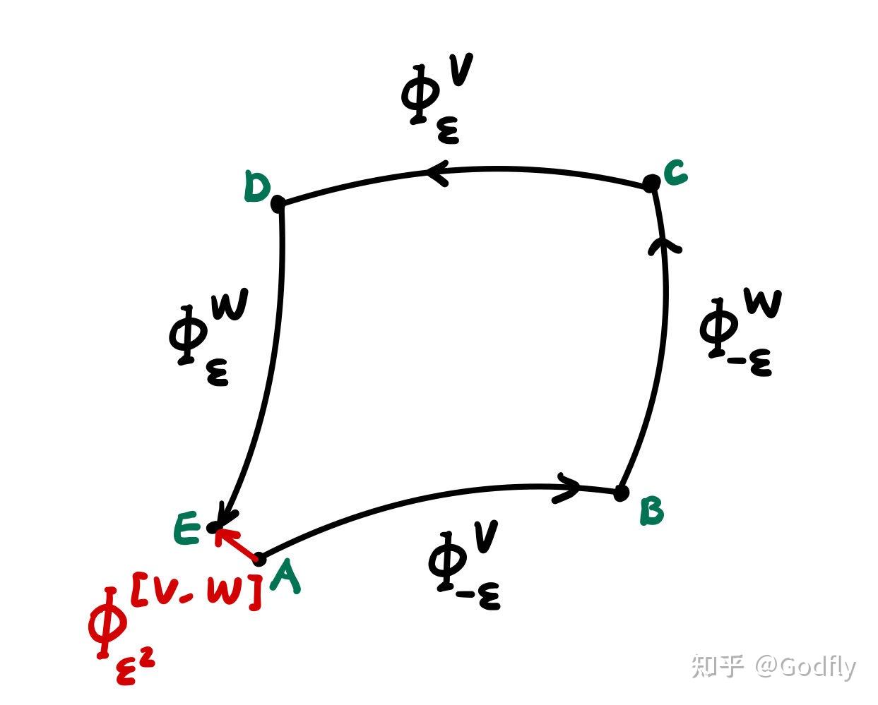
The geometric meaning of [V,W]

This reveals the geometric meaning of \([V,W]\).

If the commutator of the coordinate basis \([e^i, e^j] = 0\), the coordinate system is called holonomic; otherwise, it is non-holonomic. A non-holonomic coordinate system cannot be represented by differentiation along coordinate lines. This is because differentiation along coordinate lines satisfies \([\partial^i, \partial^j]=0\) and is therefore necessarily holonomic.

Remark

With this language, we can give another, better definition of the curvature tensor defined in Section 4.5:

Consider the loop in the figure above and transport a tensor along this loop back to the starting point. It can be shown that the transport operator can be written as

\( \tau_{A\rightarrow B\rightarrow C \rightarrow D \rightarrow E \rightarrow A} = 1 - \epsilon^2 R(V,W) \)

where

\( R(V,W) := \nabla_V\nabla_W - \nabla_W\nabla_V - \nabla_{[U,V]} \)

is the Riemann curvature tensor.

4.10 Killing Vector Fields

In Section 4.2, we imposed the requirement of metric compatibility on the covariant derivative, thereby constraining it to some extent. Together with the torsion-free condition, this uniquely determines a connection, called the RLC connection.

Can we impose a similar constraint on the Lie derivative? The answer is that doing so leads to an “overconstrained” system: given a metric, we cannot guarantee the existence of a Lie derivative that preserves it. The vector field associated with a Lie derivative having this property is called a Killing vector field. Denote a Killing vector field by \(\xi\); it satisfies the Killing equation:

\[ \mathcal{L}_{\xi} g = 0 \]

According to Example 4.11, its component form is:

\[ \xi^k g_{ij,k} + \xi^k_{,i}g_{kj} + \xi^k_{,j}g_{ik} = 0 \]

Since \(g_{ij}=g_{ji}\), the Killing equations comprise \(n(n+1)/2\) equations. However, there are only \(n\) free variables (namely, \(\xi^k, k=1,...,n\)), so this is an “overconstrained” system of equations and is not guaranteed to have a solution.

Example 4.15 Find the Killing vector fields of Euclidean space \(\mathbb{R}^2\).

The solution is \(e_1=\partial_x, e_2=\partial_y, e_3=-y\partial_x + x\partial_y\).

In addition, if we require only conformality, i.e., angle preservation, then it suffices to satisfy:

\[ \mathcal{L}_{\xi} g = \chi g, \quad \chi \in \mathcal{F}(M)\]

The equation above is called the conformal Killing equation.

Summary

In this chapter, we introduce two types of derivatives: the covariant derivative and the Lie derivative. The covariant derivative describes connections on manifolds and can be used to define parallel transport, geodesics, and curvature. Based on these concepts, we can give a brief introduction to general relativity;

The Lie derivative describes the “flow” of vector fields on a manifold. It leads to holonomy and Killing vector fields: the former characterizes whether a flow is path-dependent, while the latter characterizes whether a flow preserves the metric. Using the Lie derivative, we can define concepts such as curvature, torsion, and divergence more elegantly. In addition, it is related to Lie groups and Lie algebras, although we will not discuss them here.

Chapter 5 Integration on Manifolds

In Chapter 3, we studied differential forms on manifolds. In this chapter, we study how to integrate differential forms on manifolds.

First, we define what the “domain” of integration is. For example, in elementary calculus, we can integrate over curves as well as surfaces. The generalizations of such “domains” on manifolds are cells, simplices, and chains. Based on them, we can also define the boundary operator.

Next, we give a definition of the integral of a differential form and then introduce the celebrated Stokes’ theorem. This theorem gives the relationship between the boundary operator and the exterior derivative operator.

Finally, having introduced the boundary operator, the exterior derivative operator, and Stokes’ theorem, we must mention homology and cohomology. Homology and cohomology theory connects all the above concepts in a remarkable way and uses them to deal with “holes” in manifolds.

5.1 Cells, Simplices, and Chains (Cell, Simplex, Chain)

An m-dimensional cell (m-cell) \(\sigma\) is a parameterized m-dimensional region on an n-dimensional manifold; it is the image \(\sigma=\mathrm{Im}(\phi)\) of the map \(\phi:[0,1]^m\rightarrow M\).

It can also be understood as follows: an m-cell assigns a parameter to every point in an m-dimensional region on the manifold \(M\): \(\bm{u}\in[0,1]^m\).

We say that this m-dimensional region is embedded in the n-dimensional manifold. Equivalently, it is an m-dimensional hypersurface on the n-dimensional manifold.

Example 5.1

A point on a manifold is a 0-cell. A 0-cell is a special case: the region it represents consists of just a single point.

A curve on the 2-sphere \(S^2\) is a 1-cell (you may think of the 30° north latitude line on a globe). We assign a parameter \([0,1]\rightarrow S^2\) to every point on this curve. Clearly, not every point corresponds to a unique parameter. If the curve intersects itself, the intersection point corresponds to two distinct parameters \(u_1\neq u_2\in [0,1]\).

A surface in the manifold \(M=\mathbb{R}^3\) is a 2-cell. We assign a set of parameters \([0,1]\times[0,1]\rightarrow \mathbb{R}^3\) to every point on this surface.
More specifically, consider one-eighth of the unit sphere in the first octant. We can assign parameters as follows: \(\phi:[0,1]^2\rightarrow\mathbb{R}^3\), such that \(\phi(u,v)\rightarrow \left(\cos(\frac{\pi}{2} u)\sin(\frac{\pi}{2} v), \sin(\frac{\pi}{2} u)\sin(\frac{\pi}{2} v), \cos(\frac{\pi}{2} v)\right)\).

Remark

In Section 1.8, we specified an open cover and coordinate systems (an atlas) for the manifold \(M\). The “parameters” discussed here and the “coordinates” discussed there are two different concepts. “Parameters” are assigned to points on an m-dimensional surface embedded in an n-dimensional manifold, whereas “coordinates” are assigned to all points of the manifold itself.

In the preceding example, we can use the two parameters \(u\) and \(v\) to represent points on one-eighth of the unit sphere. However, the manifold \(\mathbb{R}^3\) in that example itself has the natural coordinate \(\mathrm{id}:\mathbb{R}^3\rightarrow\mathbb{R}^3\), which is an identity map.

There is another type of parameterization, called an m-simplex (plural: m-simplices). Unlike an m-cell, which uses the rectangular region \([0,1]^m\), it uses the triangular region \(\{(\theta_0,\theta_1,\cdots,\theta_m)\mid\sum_i\theta_i=1,\, \theta_i\ge 0\}\). This triangular region is called the standard simplex in \(\mathbb{R}^m\). Its image on the manifold under \(\varphi\) is an m-simplex on the manifold.

Remark

From the perspective of computing integrals, m-cells are more convenient; however, m-simplices are more convenient when considering topological and geometric properties. For example, we can triangulate a manifold, which is often much more convenient than working with rectangles, as shown below:

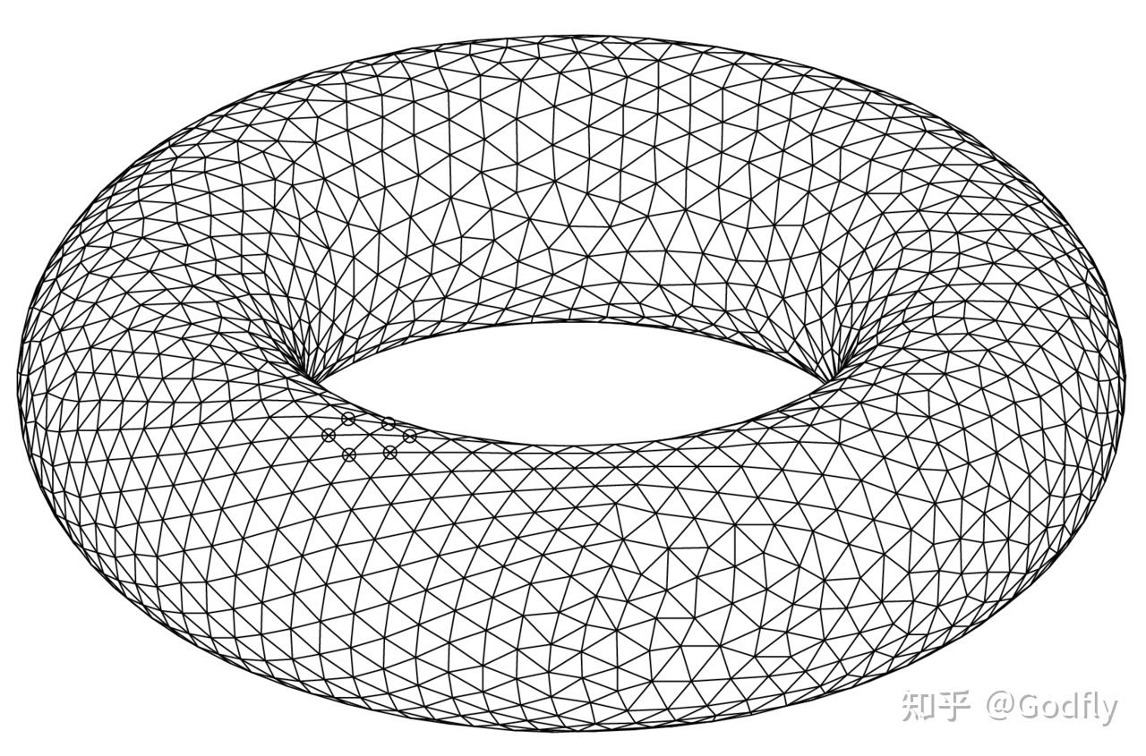
Triangulation

An m-chain is a linear combination of a collection of m-cells (or m-simplices):

\[c=\sum_i m_i\sigma_i,\quad m_i\in \mathbb{Z}\]

The set of m-chains is denoted by \(C_m(M)\).

Remark

You may now be wondering what \(c=\sum_i m_i\sigma_i\) actually means—that is, what it means to add two m-cells together. Do not worry; we will explain the meaning of this linear combination in Section 5.3. For now, you only need to regard it as a formal linear combination.

In addition, note that the coefficients in the linear combination can only be integers. Thus, \(C_m(M)\) is not a vector space, but rather a module. The difference between a module and a vector space is that scalar multiplication in a module is over \(R\times V \rightarrow V\), rather than \(F \times V \rightarrow V\), where \(R\) denotes a ring and \(F\) denotes a field. Since the integers do not form a field but only a ring, \(C_m(M)\) is a module.

5.2 Boundary Operator (Boundary Operator)

Remark

We now consider how to define the boundary of a region. With the concepts of cells/simplices and chains, we can formally define “boundary.”

Consider an (m+1)-cell, namely the image \(\sigma = \mathrm{Im}(\phi)\) of the map \(\phi: [0,1]^{m+1} \rightarrow M\). Its boundary \(\partial \sigma\) is defined as the following m-chain:

\[ \sum_{i=0}^{m}(-1)^i [\phi(x_0,\cdots,x_{i-1},1,x_{i+1},\cdots,x_{m}) - \phi(x_1,\cdots,x_{i-1},0,x_{i+1},\cdots,x_{m})] \]

The boundary of an m-chain (\(c_i\sigma_i\)) is defined as

\[\partial(c_i\sigma_i):=c_i\partial(\sigma_i).\]

We call \(\partial: C_{m+1}(M)\rightarrow C_{m}(M)\) the boundary operator.

Example 5.2

The boundary of a 1-cell (a curve) \(\phi: [0,1]\rightarrow M\) is a 0-chain: \(\phi(1) - \phi(0)\).

Here, \(\phi(1) - \phi(0)\) is an abstract linear combination of two points (0-cells).

In particular, if this curve (1-cell) is closed, i.e., \(\phi(1)=\phi(0)\), then its boundary is zero.

Thus, when we say that a closed curve has no “boundary,” we are in fact saying that its boundary is zero.

Example 5.3

Consider a 2-cell on the manifold \(\mathbb{R}^2\): \(\phi: [0,1]\times [0,1] \rightarrow \mathbb{R}^2\), \(\phi(r,\theta) = (r\cos \theta, r\sin \theta)\). It is in fact a quarter disk in the first quadrant.

The boundary of this 2-cell is the following 1-chain:

\( (\phi(1,\theta)-\phi(0,\theta)) - (\phi(r,1) - \phi(r,0)) \)

As can be seen, these four 1-cells correspond respectively to the quarter-circle arc, the origin, the radius in the \(y\) direction, and the radius in the \(x\) direction. They do indeed form the “boundary” of this quarter disk. If we interpret the signs as orientations, we also obtain an oriented loop.

The boundary can also be defined in the language of simplices. If an m-simplex is denoted by

\[ \langle p_0 ,\cdots, p_m \rangle \]

where \(p_0, \cdots, p_m\) denotes the vertices of the simplex (that is, the images of the vertices of the standard simplex), then the boundary of this m-simplex is the following (m-1)-simplex:

\[ \partial(\langle p_0 ,\cdots, p_m \rangle) := \sum_i^m (-1)^i \langle p_0 ,\cdots, p_{i-1}, p_{i+1}, \cdots, p_m \rangle \]

Thus, m-cells and m-simplices are two parallel languages.

Like the exterior derivative operator, applying the boundary operator twice also yields zero:

Theorem 5.1

\(\partial\partial=0\). Proof omitted.

5.3 Integration of Differential Forms (Integration of Differential Forms)

Remark

Whenever we integrate a differential form, we must specify a “domain” of integration. This “domain” is the m-cells / m-chains introduced in Section 5.1.

Recall that an m-cell, denoted by \(\sigma\), is the image \(\mathrm{Im}(\phi)\) of the map \(\phi:[0,1]^m\rightarrow M\). It is in fact a \(m\)-dimensional hypersurface in a \(n\)-dimensional manifold. Next, we define the integral of a differential form over an m-cell.

In differential geometry, the definition of integration involves the concept of the pullback map (see Section 4.7). Specifically, the integral of \(\omega\) over \(\sigma\) is defined as the multiple integral of \(\phi^*\omega\) over \([0,1]^m\). Here, \(\phi^*\omega\) indicates that the map \(\phi\) pulls \(\omega\) back from the region \(\sigma\) on the manifold to the region \([0,1]^m\subseteq \mathbb{R}^m\) in \(\mathbb{R}^m\). In other words, \(\phi^*\omega\) is a differential form on \(\mathbb{R}^m\).

We now summarize the above relation in mathematical notation:

\[ \int_{\sigma} \omega = \int_{\phi[D]} \omega := \int_{D} \phi^{*} \omega \]

Here, \(\phi[D]\) denotes an m-cell or an m-simplex, depending on whether you use the language of cells or that of simplices. For example, in the case of cells, \(D\) denotes a rectangular region \([0,1]^m \in \mathbb{R}^m\).

Remark

Since a differential form can be regarded as an antisymmetric tensor field of type \((0,q)\), the pullback map introduced in Section 4.7 can certainly be applied to a differential form.

We now give an explicit formula for the integral of a differential form over an m-cell.

As noted at the end of Section 3.3, we may write a differential form \(\omega\) as:

\[ \begin{aligned} \omega = \sum_{i_1\lt \cdots\lt i_m} f_{(i_1,\cdots,i_m)}\mathrm{d}x^{i_1}\wedge\cdots\wedge\mathrm{d}x^{i_m} \end{aligned} \]

For definiteness, we may stipulate that \((i_1, \cdots, i_m)\) is an even permutation of \((1, \cdots, m)\).

Then the integral of \(\omega\) over \(\sigma\) can be written explicitly as:

\[ \begin{aligned} \int_\sigma \omega=\int_{[0,1]^m}\sum_{i_1\lt \cdots\lt i_m} f_{(i_1,\cdots,i_m)}|_{\phi( \mathbf{u})}\frac{\partial(x^{i_1},\cdots,x^{i_m})}{\partial(u^1,\cdots,u^m)}\mathrm{d}u^1\cdots\mathrm{d}u^m \end{aligned} \]

where \((u^1,\cdots,u^m)\in[0,1]^m\); \(\frac{\partial(x^{i_1},\cdots,x^{i_m})}{\partial(u^1,\cdots,u^m)}\) is the Jacobian determinant:

\[\begin{aligned} \frac{\partial(x^{i_1},\cdots,x^{i_m})}{\partial(u^1,\cdots,u^m)} := \begin{vmatrix} \frac{\partial x^{i_1}}{\partial u^1} & \cdots & \frac{\partial x^{i_1}}{\partial u^m} \\ \vdots & \ddots & \vdots \\ \frac{\partial x^{i_m}}{\partial u^1} & \cdots & \frac{\partial x^{i_m}}{\partial u^m} \end{vmatrix} \end{aligned}\]

Notice that the right-hand side is an ordinary multiple integral, which was thoroughly discussed when we studied elementary calculus, so we will not repeat that discussion here.

Remark

Deriving an explicit expression for the integral from its definition requires some computation.

Specifically, we first need to recall the pullback of a tensor field of type \((0,n)\), introduced in Section 4.7:

\( \begin{aligned} \phi^*: \mathcal{T}^0_l(N) &\rightarrow \mathcal{T}^0_l(M) \\ \phi^*T(v^1|_p, \cdots, v^n|_p) &:= T((\phi_* v^1)|_{\phi(p)}, \cdots, (\phi_* v^n)|_{\phi(p)}) \end{aligned} \)

and derive its explicit form:

\( \phi^*(\mathrm{d}y^k \otimes \cdots \otimes \mathrm{d}y^l) = J^k_i \cdots J^l_j \mathrm{d}x^i \otimes \cdots \otimes \mathrm{d} x^j \)

Second, we need to prove that, for an \(n \times n\) matrix \(A\), its determinant satisfies:

\( \operatorname{det} A = \epsilon_{k...l} A^k_1 \cdots A^l_n \)

where \(\epsilon\) is the generalized Levi-Civita symbol; \(\epsilon_{12...n} = 1\), and interchanging any two indices reverses its sign. This is simply another way of writing the usual definition of the determinant.

Finally, we can derive the formula for the pullback of a differential form:

\( \begin{aligned} \phi^*(\mathrm{d}x^{i_1}\wedge\cdots\wedge\mathrm{d}x^{i_m}) &= \phi^* \left(\frac{1}{p!} \epsilon_{i_1...i_m} \mathrm{d}x^{i_1}\otimes\cdots\otimes\mathrm{d}x^{i_m}\right)\\ &= \frac{1}{p!} \epsilon_{i_1...i_m}J^{i_1}_{1} \cdots J^{i_m}_{m} \mathrm{d}u^1 \otimes \cdots \otimes \mathrm{d}u^m \\ &= \epsilon_{i_1...i_m} J^{i_1}_{1} \cdots J^{i_m}_{m} \mathrm{d}u^1 \wedge \cdots \wedge \mathrm{d}u^m \\ &= (\operatorname{det} J) \mathrm{d}u^1 \wedge \cdots \wedge \mathrm{d}u^m \end{aligned} \)

where \(\operatorname{det} J\) is the determinant of the Jacobian matrix, or simply the Jacobian determinant.

From the formula above, we can derive the formula in the main text.

Remark

We have now defined the integral of differential forms over m-cells. Next, we define the integral of differential forms over m-chains.

The integral of an \(m\)-form \(\omega\) over an m-chain (\(c=\sum_i c_i\sigma_i\)) is defined as follows:

\[ \begin{aligned} \int_c\omega=\sum_i c_i\int_{\sigma_i}\omega \end{aligned} \]

where \(\sigma_i\) is an m-cell.

5.4 Stokes’ Theorem

With the concepts developed in the preceding sections, we can now introduce the celebrated Stokes’ theorem.

Stokes’ Theorem

Given an (m+1)-chain \(c\in C_{m+1}\) and an m-form \(\alpha \in \bigwedge^m(T^*M)\), we have

\[\begin{aligned} \int_c \mathrm{d} \alpha = \int_{\partial c} \alpha \end{aligned}\]

Let us now see how Stokes’ theorem reduces to familiar forms.

Example 5.4 Fundamental Theorem of Calculus

\( \int_a^b f^\prime(x)\mathrm{d}x = f(b) - f(a) \)

This follows from Stokes’ theorem by taking \(M=\mathbb{R}^1\) and \(c = [a,b]\).

Example 5.5 Green’s Theorem

\( \iint_D \left( \frac{\partial Q}{\partial x} - \frac{\partial P}{\partial y}\right) \mathrm{d}x\mathrm{d}y = \oint_{\partial D} (P\mathrm{d}x+Q\mathrm{d}y) \)

This follows from Stokes’ theorem by taking \(M=\mathbb{R}^2\), \(c = D\), and \(\alpha = P\mathrm{d}x+Q\mathrm{d}y\).

Example 5.6 Gauss’s Theorem

\(\begin{aligned} \int_{D}(\operatorname{div} V)\omega_g = \int_{\partial D} V^i \mathrm{d} \Sigma_i|_{\partial D} \end{aligned}\)

Here \(\omega_g\) is the volume form of unit volume with respect to the metric \(g\), and

\( \mathrm{d}\Sigma_i := \frac{1}{(n-1)!} \omega_{ij...k} \mathrm{d}x^j\wedge \cdots \wedge \mathrm{d}x^k \)

Hint: Since \((\operatorname{div} V)\omega_g =: \mathcal{L}_V \omega_g\), by Stokes’ theorem it suffices to prove \(\mathcal{L}_V \omega_g = \mathrm{d}(V^i\mathrm{d}\Sigma_i)\).

5.5 *Introduction to Homology & Cohomology

Remark

To some extent, manifolds can be classified by the number and types of their “holes.” This is commonly used to illustrate the idea in popular introductions to topology.

Homology was developed to study “holes.” How do we define a “hole”?

Observe that on a manifold without holes, a hypersurface or curve without boundary—i.e., one that is closed—must be the boundary of another region. In other words, a p-chain with zero boundary (see Section 5.2) is always the boundary of some (p+1)-chain.

However, this does not hold on a manifold with holes. Imagine a chain that goes once around a torus and joins end to end: its boundary is zero, but it is not the boundary of any chain.

Remark

Of course, if a chain is the boundary of another chain, then its own boundary must be zero, because \(\partial\partial=0\) (Theorem 5.1).

Mathematically, we can define this class of objects in the language of algebra:

\[\begin{aligned} H_p(M) := \frac{ \{c_p \mid \partial c_p=0\} }{ \{c_p \mid \partial c_{p+1} = c_p \} } \end{aligned}\]

where \(c_p\) denotes a p-chain.

Remark

Or, more rigorously:

\(\begin{aligned} H_p(M) := \frac{ \{c \in C_p \mid \partial c=0\} }{ \{c \in C_p \mid \partial c^{\prime} = c; c^{\prime} \in C_{p+1} \} } \end{aligned}\)

If these symbols are confusing, return to Section 5.2.

or equivalently,

\[\begin{aligned} H_p(M) := \frac{\operatorname{Ker} \partial_{p}}{\operatorname{Im} \partial_{p+1}} \end{aligned}\]

\(H_p(M)\) is called the \(p\)th homology group; it is a quotient group of two groups. An element of a homology group is called a homology class.

Remark

For example, the homology class of \(S_1\) (a closed curve) is \(\mathbb{Z}\). This is because one may wind around once, twice, three times, and so on; one may also wind around an integer number of times in the opposite direction. Of course, one may also not wind around at all. This corresponds to the group of integers.

The first homology group of a torus (mathematically defined as \(T:=S^1\times S^1\)) is \(\mathbb{Z} \times \mathbb{Z}\). This is fairly intuitive both algebraically and geometrically; see the figure below:

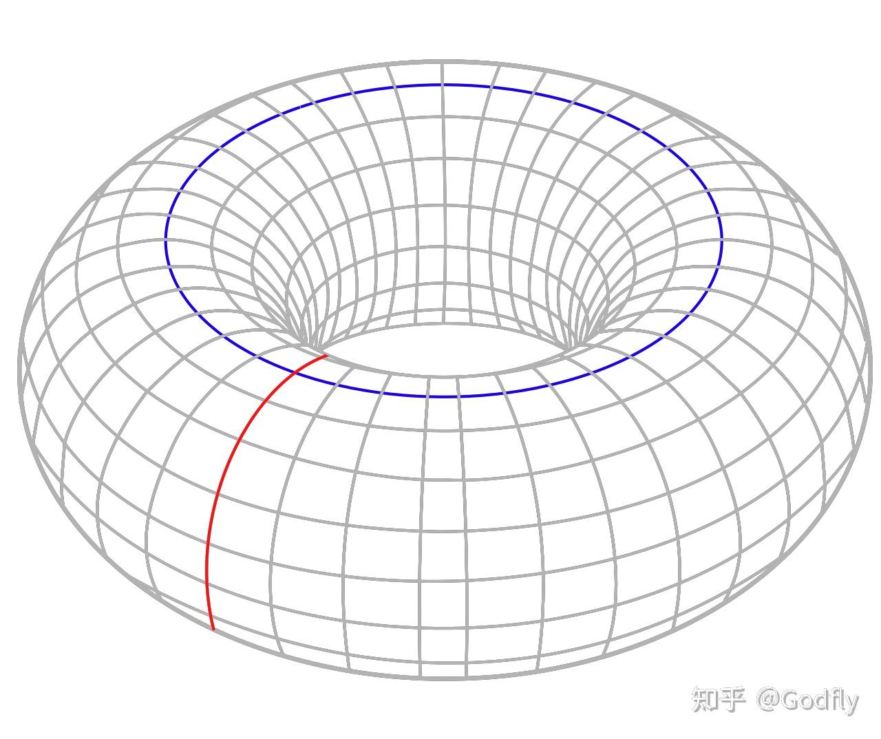
The homology group of a torus is ZxZ. As can be seen intuitively from the figure, there are two distinct ways to wind around it.

Let us now consider what cohomology is concerned with. In physics, we usually assume that every closed form is exact. For example, from the fact that the curl of an electric field (see Sections 3.4–5) is zero, we infer the existence of an electric potential; and from the fact that the divergence of a magnetic field (see Sections 3.4–5) is zero, we infer the existence of a magnetic potential.

Remark

An exact form is a form that is the (exterior) differential of another form.

A closed form is a form whose (exterior) differential is zero.

However, this need not hold on a general manifold. There may be a form whose differential is zero but which is not the differential of any form. In other words, there exist closed forms that are not exact.

Remark

Imagine the lateral surface of a cylinder (\(\mathbb{R}^1 \times S^1\)) carrying a uniform electric field that circulates once around it. It can be shown that such an electric field is divergence-free, but it is not conservative: if an electron travels once around in the direction of the electric field and returns to its original position, its energy decreases. In this case, the electric potential is not well defined.

Why, then, do we assume in ordinary physics that electric and magnetic potentials always exist? It is because we believe that the space we inhabit has no “holes.” In other words, in a simply connected space (recall multivariable calculus), the vanishing differential of a form implies that it is exact.

Cohomology is concerned with the following questions: when is a closed form exact, and how many classes of closed forms are not exact?

Remark

Conversely, every exact form is necessarily closed, because \(\mathrm{dd} = 0\) (Theorem 3.1).

The (de Rham) cohomology group can be defined as “all exact forms” modulo “all closed forms,” namely:

\[\begin{aligned} H^p(M) = \frac{ \{ \omega \mid \mathrm{d}\omega = 0 \} }{ \{ \omega \mid \mathrm{d} \alpha = \omega\} } \end{aligned}\]

or equivalently,

\[\begin{aligned} H^p(M) = \frac{\operatorname{Ker}\mathrm{d}_p}{\operatorname{Im}\mathrm{d}_{p-1}} \end{aligned}\]

\(H^p(M)\) is called the \(p\)-th cohomology group, whose elements are called cohomology classes. Cohomology groups tell us how many classes of closed forms that are not exact forms there are.

Finally, there is a theorem that connects homology and cohomology: Poincaré duality:

Poincaré Duality

For an n-dimensional orientable, compact manifold without boundary, its k-th homology group is isomorphic to its (n-k)-th cohomology group, namely

\[H^k(M)\cong H_{n-k}(M)\]

Strictly speaking, the cohomology here is singular cohomology \(H^k(M;\mathbb{Z})\) rather than de Rham cohomology \(H^k_{\text{dR}}(M)\), the latter of which is isomorphic to \(H^k(M;\mathbb{R})\).

In other words, there is a natural one-to-one correspondence between the equivalence classes of the following two objects:

Forms that are not the differential of another form, but whose own differential is zero

Chains that are not the boundary of another chain, but whose own boundary is zero

Save, Like, and Keep the Good Luck Coming

If you found this article helpful, please give it a like~