What Is a Differential?
 Haifei
I. Is a Differential an Infinitesimal?
Physicists like to regard a differential as a very small quantity. This is always convenient in calculations, but it gives one a feeling of imprecision.
In fact, it is indeed imprecise; the second mathematical crisis arose for this reason.
Rigor and accessibility are forever complementary. Regarding a differential as an infinitesimal caters to intuitive sensibilities, yet cannot pass rational scrutiny.
II. A Differential Is a Linear Function
I prefer to think of a differential (at a certain point) as a machine. For example,
\[f:f(x,y)=x^2+2y^2\]The differential at \((1,1)\)
is such a machine:
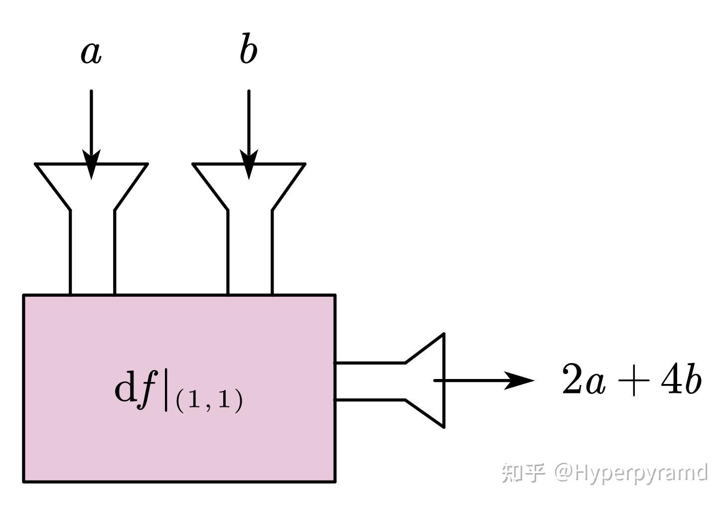
It takes two numbers and outputs one number.
Written out, it looks like this:
\[\mathrm{d}f|_{(1,1)}(a,b)=\frac{\partial f}{\partial x}\bigg|_{(1,1)}a+\frac{\partial f}{\partial y}\bigg|_{(1,1)}b=2a+4b\]Since the partial derivatives at each point may differ, if we say that the differential at a certain point is a machine, then differentials are an ocean of machines.
You may also have noticed that this machine is “linear”; it is simply a linear map from \(\mathbb{R}^2\) to \(\mathbb{R}\).
Knowledge from linear algebra tells us that the set of linear functions forms a linear space. In other words, linear functions themselves are “vectors”: they can be added, subtracted, and multiplied by scalars.
Returning to the analogy above, this means that we can add two machines together: \(\mathrm{d}f|_p+\mathrm{d}g|_p\),
and we can also make one machine \(\lambda\) times as large as before: \(\lambda \cdot \mathrm{d}f|_p \).
The subscript p denotes evaluation at the point p.
What does it mean to add machines together? For example, if
\(\mathrm{d}f|_p(a,b)=2a+4b,\,\, \mathrm{d}g|_p(a,b)=a-b\),
then \(\mathrm{d}f|_p(a,b)+\mathrm{d}g|_p(a,b)=3a+3b\).
This is much like adding two vectors: \((2,4)+(1,-1)=(3,3)\).
In fact, they are vectors. Yes, you heard that right: differentials are vector (fields).
III. Differentials Are Dual Vector Fields / Covector Fields
3.1 Tangent Spaces
If you want to study differentials on a curved surface, then you need to redefine some concepts. For example, a differential is linear, but a manifold is curved, so we need to define something linear within this curvature. This linear object is the tangent space.
As the name suggests, a tangent space is the tangent plane to a curved surface at a certain point. But how should it be defined? The curvature here is not curvature embedded in another space, but rather curvature of space itself; this curvature is intrinsic. We cannot find the equation of a tangent plane as in classical analytic geometry.
Let us take another approach:
First, it is linear, meaning that it is a vector space.
A vector space is an Abelian group equipped with scalar multiplication. Specifically, its elements (called vectors) satisfy the following properties:
(1)Commutativity of vector addition
(2)Associativity of vector addition
(3)Vector addition has an identity element (analogous to zero)
(4)Vector addition has inverse elements (analogous to additive inverses)
The above four properties indicate that a linear space is an Abelian group with respect to vector addition.
(5)Scalar multiplication has a multiplicative identity element
(6)Associativity of scalar multiplication
(7)Distributivity of scalar multiplication (over scalars)
(8)Distributivity of scalar multiplication (over vectors)
A vector space need not be \(\mathbb{R}^n,\,\mathbb{C}^n\). As long as addition and scalar multiplication are defined on a set and satisfy the above properties, that set is a vector space.
We can define such a vector space whose elements are linear maps from the set of smooth functions to the real numbers:
\(v:\mathcal{F}_M\rightarrow\mathbb{R}\) satisfies
(1)\(v(\lambda f+\mu g)=\lambda v(f)+\mu v(g)\) (linearity)
(2) \(v|_p(f\cdot g)=f|_p\cdot v(g)+g|_p\cdot v(f)\) (the Leibniz rule)
where \(\mathcal{F}_M\) is the set of all smooth functions on the differentiable manifold \(M\).
It can be proved that the set of \(v\) forms a vector space.
Do not be intimidated by this complicated definition; in fact, it is just the directional derivative of a function at a certain point.
Taking a function of two variables as an example, let us explicitly write out an instance of \(v\): \(\left(a\frac{\partial}{\partial x}+b\frac{\partial}{\partial y}\right)\bigg|_p\)
If \((\frac{\partial}{\partial x}\bigg|_p,\frac{\partial}{\partial y}\bigg|_p)\) is taken as the basis, then its coordinates are \((a,b)\).
This linear space is the tangent space at the point \(p\) on the manifold \(M\), denoted by \(T_pM\).
All the operations above are at a certain point \(p\); a tangent space grows out of every point. You can imagine every point on a curved surface growing its own tangent plane.
We can abbreviate \(\frac{\partial}{\partial x}\) as \(\partial_x\), and abbreviate \(\frac{\partial}{\partial y}\) as \(\partial_y\).
3.2 Cotangent Spaces
We have just introduced the tangent space \(T_p M\). We now call the dual space \(T_p^*M\) of the tangent space the cotangent space.
The differential at a certain point is precisely an element of the cotangent space. In other words, the differential at a certain point is a cotangent vector.
Elements of a dual space (cotangent vectors) are linear functionals that can map elements of the original space to a number. This is precisely the machine we mentioned earlier:
Except that the input should now be an element \(\left(a\partial_x+b\partial_y\right)|_p\) of the tangent space.
As we have said, differentials are an ocean of machines. Therefore, an ocean of cotangent vectors (that is, differentials) may be called a cotangent vector field.
In mathematics, a differential (cotangent vector field) has a cool name: a section of the cotangent bundle. See
An Introduction to Differential Geometry (Physicist’s Version)
After all this abstract talk, let us now give a definition:
The differential at a point \(p\) on a manifold \(M\) is a linear functional which acts on an element \(v|_p\in T_pM\) of the tangent space and yields \(\mathrm{d}f|_p(v|_p)=v|_p(f)\)
Let us give a more explicit example, again using a function of two variables:
\[\mathrm{d}f|_{p}:\mathrm{d}f|_{p}(v|_p)=v|_p(f)= (\partial_x f)|_{p}\cdot a+(\partial_y f)|_{p}b,\quad \text{where}\quad v|_p=\left(a\partial_x+b\partial_y\right)|_p\]Vectors in the tangent space can also be called covariant vectors, and vectors in the cotangent space can also be called covariant vectors. What is going on here?
Contravariant vectors
Before encountering differential geometry, we were basically using contravariant vector fields rather than covariant vector fields. This is because, once we choose a basis, a coordinate transformation is the inverse transformation of the basis transformation. This is what “contravariant” means: the transformation rule is opposite to that of the basis transformation.
For example, given a vector field \(A^\mu = (A^x, A^y, A^z)\), namely \(A = A^\mu e_\mu\), where \(e_\mu\) is the basis we have chosen. Note that Einstein summation convention is used here, meaning that repeated upper and lower indices are summed over.
When making the basis transformation \(e^\prime_\nu = M^{\mu}_\nu e_{\mu}\), since \(A^\mu e_\mu = A^{\prime \mu} e^\prime_\mu\), clearly the coordinate transformation should be \(A^{\prime \mu} = (M^{-1})^{\mu}_{\nu} A^\nu\).
In fact, \(e_\mu = \partial_\mu = \frac{\partial}{\partial x_\mu}\). This may seem strange, but in differential geometry, contravariant vectors are defined as partial derivative operators, as stated above.
Note that the coordinates of contravariant vectors should all be written with upper indices, for example \(A^\mu\), so that they can be contracted with the lower indices of the basis \(e_\mu\) (according to Einstein summation convention).
Covariant vectors
Conversely, “covariant” means that the coordinate transformation and the basis transformation have the same matrix. But how can such vectors exist?
In fact, covariant vectors live in another space, called the dual space of the original space.
A vector \(\omega_\mu\) (written with lower indices) in the dual space and a vector \(v^{\mu}\) (with upper indices) in the original space can be contracted into a scalar: \(\omega_\mu v^\mu = C\).
The basis dual to \(e_\mu = \partial_\mu\) is \(\mathrm{d}x^\mu\), satisfying \(\mathrm{d}x^\mu \partial_\nu = \delta^\mu_\nu = \begin{cases} 1 & \mu=\nu \\ 0 & \mu\ne \nu\end{cases}\).
Using reasoning similar to before, we can conclude that the transformation matrix of the dual basis \(\mathrm{d}x^\mu\) is the inverse of the transformation matrix of the basis \(\partial_\mu\). Thus, the transformation matrix for the coordinates \(\omega_\mu\) of dual vectors is the inverse of the inverse of the transformation matrix for the basis \(v^\mu\), and is therefore exactly equal to the basis transformation matrix itself.
This is what “covariant” means: the transformation rule is the same as that of the basis transformation.
Therefore, we can also say that differentials are covariant vector fields.
IV. Differential Forms Are Antisymmetric Covariant Tensor Fields / Antisymmetric Multilinear Functionals
Differential forms can be regarded as covariant antisymmetric tensor fields. Antisymmetry means that exchanging indices changes the sign: \(\omega_{\mu \nu} = -\omega_{\nu\mu}\).
For example, a second-order antisymmetric covariant tensor field \(\omega_{\mu\nu}\) is a 2-form.
In particular, a covariant vector field (that is, what we usually call a differential) \(\omega_\mu\) is a 1-form, while a scalar field is a 0-form.
Two 1-forms can produce a 2-form through the wedge product:
\[\omega = \alpha \wedge \beta = \alpha_\mu \beta_\nu\mathrm{d}x^\mu \wedge \mathrm{d}x^\nu \]where \(\mathrm{d}x^\mu \wedge \mathrm{d}x^\nu = -\mathrm{d}x^\nu \wedge \mathrm{d}x^\mu\)
And so on.
The differentials discussed before this section are all 1-forms. A 1-form (at a certain point) is a linear functional from the tangent space to the real numbers, but what is an n-form?
An n-form (at a certain point) is defined as an antisymmetric multilinear functional with n inputs. Antisymmetry means that exchanging two inputs adds a minus sign to the output:
\[\omega^1\wedge \omega^2\wedge\cdots\wedge \omega^n(v_1,v_2,\cdots,v_n)= \begin{vmatrix} \omega^1(v_1) & \cdots & \omega^{1}(v_n) \\ \vdots & \ddots & \vdots \\ \omega^n(v_1) & \cdots & \omega^n(v_n) \end{vmatrix}\]According to the properties of determinants, exchanging two columns changes a determinant to its negative. This perfectly characterizes the antisymmetry of differential forms.
Example:
At a point \(p\) on a 3-dimensional manifold, there is a 2-form: \(\omega = 5\mathrm{d}x^1 \wedge \mathrm{d}x^3 -2\mathrm{d}x^2\wedge \mathrm{d}x^3\)
Acting on two tangent vectors \(u=\partial_1+2\partial_2+3\partial_3\) and \(v=3\partial_1-2\partial_2+\partial_3\) yields:
\[\begin{aligned} \omega(u,v)&= 5\begin{vmatrix} \mathrm{d}x^1(\partial_1+2\partial_2+3\partial_3) & \mathrm{d}x^1(3\partial_1-2\partial_2+\partial_3) \\ \mathrm{d}x^2(\partial_1+2\partial_2+3\partial_3) & \mathrm{d}x^2(3\partial_1-2\partial_2+\partial_3) \end{vmatrix}\\ &-2\begin{vmatrix} \mathrm{d}x^2(\partial_1+2\partial_2+3\partial_3) & \mathrm{d}x^2(3\partial_1-2\partial_2+\partial_3) \\ \mathrm{d}x^3(\partial_1+2\partial_2+3\partial_3) & \mathrm{d}x^3(3\partial_1-2\partial_2+\partial_3) \end{vmatrix} \\&=5\cdot\begin{vmatrix}1&3\\2 &-2\end{vmatrix}-2\cdot\begin{vmatrix}2&-2\\3 & 1\end{vmatrix} \\&=-48 \end{aligned}\]Its geometric meaning is the area of the projection, onto the surface element \(\omega\), of the parallelogram formed by the vectors \(u\) and \(v\). Of course, this area is oriented, so negative values may occur.
Why do we require differential forms to have an antisymmetric structure? Because we want differential forms to describe the concept of volume. See:
Once we have the concept of volume, we can integrate differential forms. In fact, when we compute surface integrals and volume integrals in advanced mathematics, we are using differential forms:
\[\mathrm{d}x\, \mathrm{d}y \,\mathrm{d}z := \mathrm{d}x \wedge \mathrm{d}y \wedge \mathrm{d}z\]In differential geometry, we integrate differential forms rather than functions. For example, in the expression \(\int f(x) \mathrm{d}x\), \(\mathrm{d}x\) is a 1-form, and \(f(x) \mathrm{d}x\) is also a 1-form; in the expression \(\int f(x,y,z) \,\mathrm{d}x\, \mathrm{d}y \,\mathrm{d}z\), \(\mathrm{d}x\, \mathrm{d}y \,\mathrm{d}z := \mathrm{d}x \wedge \mathrm{d}y \wedge \mathrm{d}z\) is a 3-form, and \(f(x)\mathrm{d}x \wedge \mathrm{d}y \wedge \mathrm{d}z\) is also a 3-form.
V. A Differential Is an Exterior Derivative
The “differentials” discussed above all refer to another mathematical object obtained after a mathematical object undergoes a “differentiation operation.”
Then what is the “differentiation operation” itself? It is the exterior derivative.
Define the exterior derivative operation \(\mathrm{d}\), which transforms an n-form into an (n+1)-form:
\[\begin{aligned} \mathrm{d} \omega &= \mathrm{d}(\omega_\mu \mathrm{d}x^\mu)\ \\ &:= \mathrm{d}(\omega_\mu) \wedge \mathrm{d}x^\mu \\ &= (\partial_\nu \omega_\mu\mathrm{d}x^\nu)\wedge\mathrm{d}x^\mu \end{aligned}\]In a word, the exterior derivative operation takes the total differential of the component on each basis and then wedges it with the corresponding basis.
In particular, applying the exterior derivative operation to a 0-form (a scalar field) gives what we usually call a differential: \(\mathrm{d}f = (\partial_\mu f) \mathrm{d}x^\mu\).
As for the use of the exterior derivative, please see the other articles in this column. That is all for now about differentials.